
Training an Open-Source Foundation Model for Bat Acoustics Using Data from the North American Bat Monitoring Program (NABat)
This page describes the motivation, inputs, procedures, and experiments that have been performed towards a spectrogram-based foundation model for high-frequency biological datasets on bats at the U.S. Geological Survey (USGS).
1. Executive Summary
Bioacoustics are valuable inputs for monitoring the presence of acoustically active cryptic species and offer an opportunity to lower the cost of labor-intensive ecological surveys. Self-supervised learning (SSL) has emerged as a promising technique for creating generalizable machine models from large, loosely labeled or unlabeled datasets. This document describes the motivation, inputs, procedures, and experiments that have been performed towards a spectrogram-based foundation model for high-frequency biological datasets on bats at the U.S. Geological Survey (USGS).
2. Program Background
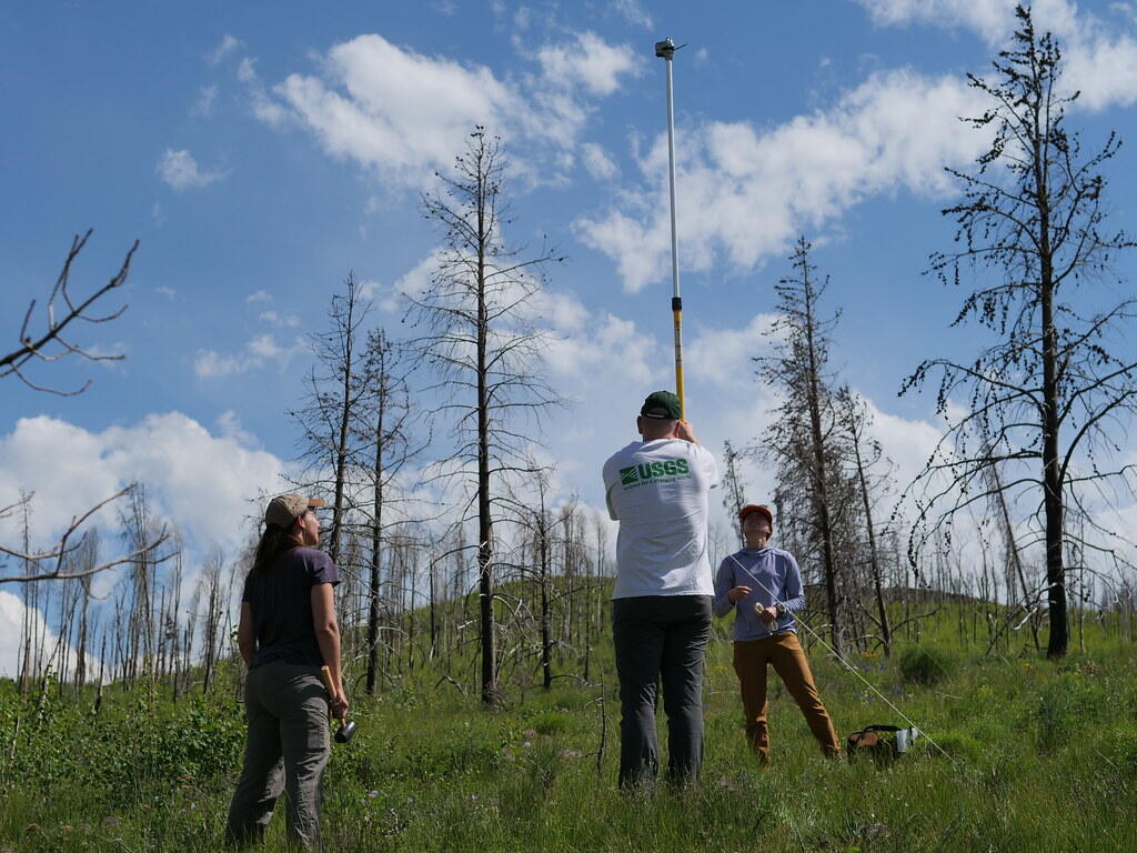
The North American Bat Monitoring Program (NABat), co-led by the USGS and U.S. Fish and Wildlife Service, is a continent-wide effort to monitor the health of bat populations through species-level status and trends analyses. As a critical component to the program, NABat depends on partners to collect and submit acoustic survey data following a spatially balanced, grid-based sample design. The program provides guidance and protocols for a range of survey types including stationary and mobile acoustic surveys, roost and emergence counts, and hand captures (Loeb et al. 2015).
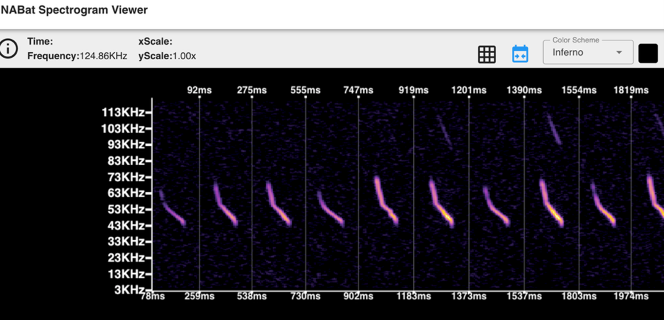
Stationary acoustic surveys are critical for bat summer population status and trends analyses (Udell et al. 2022). Surveyors deploy high-frequency recording devices for four consecutive nights to record bat echolocation calls. These calls are saved in five second chunks onto a removable storage card and are subsequently transferred to a computer for processing. Proprietary software is often used to visualize spectrograms of the call data and can also be used to assign a species classification to each recording using opaque heuristics (i.e., “auto ID”) (Reichert et al. 2018). Experts specializing in a particular species or geographic area can also assign a species classification to each call file (i.e. “manual ID”). Only a handful of vendors exist who make microphones, recorders, and processing software for bats.
To increase the quantity and quality of status and trends products, NABat aims to reduce barriers to entry for acoustic monitoring of bats. A critical component of this effort is to create and distribute open-source species classification models. These high-fidelity models will provide opportunities to more accurately model the uncertainty inherent in acoustic data in downstream statistical products.
Supervised learning with convolutional neural networks (CNN) can use spectrogram representations of full spectrum high frequency acoustic data or a highly optimized zero-crossing format that is popular with the bat biologist community. Supervised learning uses labeled datasets to build a classifier that can discriminate between categories present in training data. Unfortunately, some resulting models have been limited by the availability of high confidence training data (Khalighifar et al. 2022).
As an alternative to supervised learning, self-supervised learning (SSL) techniques can help to overcome limitations in strongly labeled training data by enabling models to learn meaningful structure directly from the data itself, without requiring explicit species labels. In computer‑vision applications, SSL methods train a model to predict or reconstruct withheld parts of an image to distinguish different augmented views of the same image. This forces the model to internalize the underlying patterns present in the full dataset (He et al. 2020). As the model learns from all available acoustic images, not just the subset with high‑confidence species annotations, it can extract richer, more generalizable representations of call structure, noise, and detector artifacts. These learned representations can improve downstream classification results, especially when combined with pretraining with large diverse labeled data or fine tuning with more task specific datasets (Schwinger et al. 2026). Downstream tasks that we are interested in evaluating with an SSL model include species classification, call quality assessment, and species classification for specific regions or recording devices.
3. Prior Work and Previous Models
NABat has used CNNs with stationary acoustic files for species detection in bats. In our first effort, we used a custom TensorFlow-based topology with a high-confidence training dataset of roughly 25,000 recordings (Khalighifar et al. 2022). We then extended this work with a subsequent data release of the training dataset and two companion software releases. These software releases included a description of our training algorithm (Gotthold et al. 2022) and a runner with a trained model for general use (Gotthold et al. 2024). This work helped us identify how limitations in the size and diversity of a training dataset can materially impact the quality of the resulting model.
To improve model quality, we, in partnership with Kitware, Inc. (Kitware, 2026) developed a MobileNet-based, PyTorch-trained model (https://github.com/Kitware/batai) using a novel spectrogram representation which creates a compressed composite of multiple pulses from full spectrum acoustic files (https://doi.org/10.5066/P969TX8F).
While full spectrum acoustic data may provide a richer source of potential information to improve model classification, models trained on zero-crossing data have also performed reasonably well (Agranat et al. 2012). Zero crossing data was prevalent in bat bioacoustics monitoring when device storage space was more limited as it only saves the dominant frequency in a time slice. To support analysis who either want access to legacy zero crossing datasets or have data storage limitations, we have created a bat species classifier using supervised learning on a MobileNet convolutional neural network (CNN). The model can be shared upon request.
4. Training Dataset for Foundation Modeling
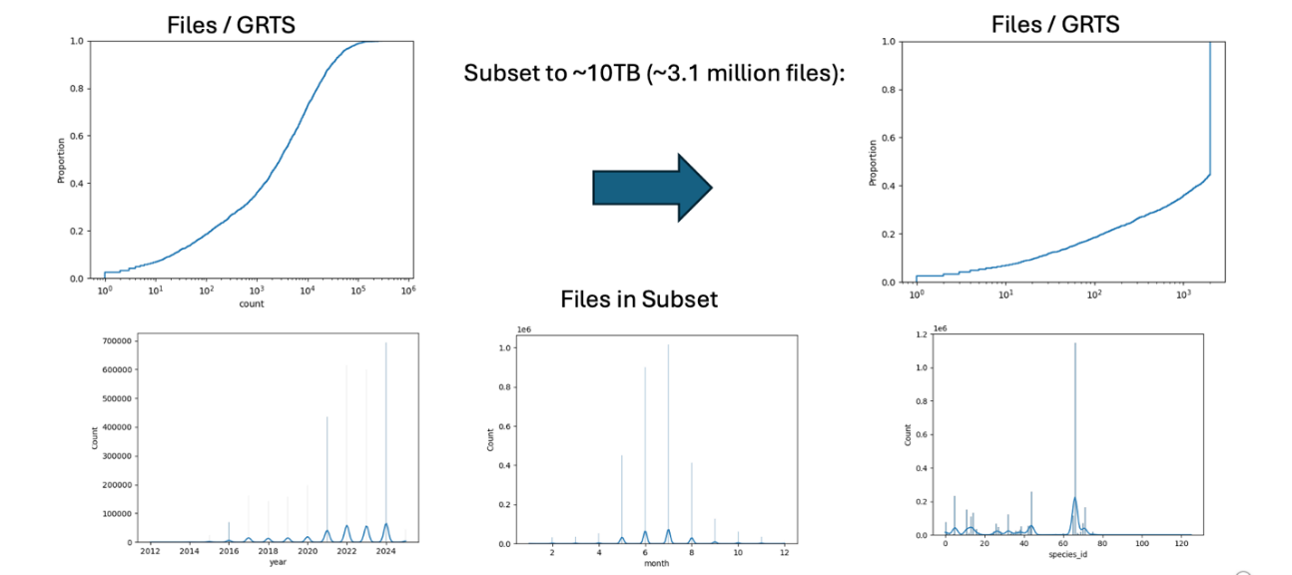
NABat has been collecting acoustic files from partners across the United States, Canada, and Mexico, since 2019. In this time, the program has now collected over 150TB of acoustic data on bats. However, training a model on this large amount of data can be cost prohibitive. As such, we sampled from the full acoustic dataset in such a manner as to preserve acoustic and geographic diversity.
We staged the partial ~10TB dataset by creating a dedicated S3 bucket in Amazon Web Services (AWS) with the appropriate policies for copying acoustic files from the AWS S3 bucket to the USGS Caldera storage system. Selected files were copied into the dedicated AWS S3 bucket using AWS Batch and then used the USGS High Performance Computing (HPC) team’s Globus connector to move the data to the destination.
TASK DETAILS
Task ID: 4cfc4308-c951-11f0-a439-0ed8a6a59ea5
Task Type: TRANSFER
Status: SUCCEEDED
Source: Hovenweep AWS S3 Storage
Destination: Hovenweep Disk Storage
Files Transferred: 3143414
Directories Transferred: 2389
Bytes Transferred: 11524345674814
Effective Speed: 44829562 Bytes per Second
Transfer Settings:
- verify file integrity after transfer
- transfer is encrypted
- quota errors prevent transfer retry
- overwriting all files on destination
We elected a 90/10% split and persisted the files in JSONL manifests for training and testing datasets. In this context, the training dataset comprises the spectrograms that we augment during the SSL training and the files in the testing dataset are held aside to ensure that we are making progress towards separating labels for the downstream supervised learning task. For the experiment below, we reserve 20,000 labeled files from the testing dataset for a linear probe which we used to score the utility of the ‘backbone’ that the SSL process is training for the downstream classification task. The backbone is the core neural network that is responsible for extracting features during training. The linear probe validation classifier takes the backbone that is being trained during the SSL process, freezes the weights and then adds a single linear layer for the labels in the test data. For this task we are using a standard 80% / 20% training / validation split of the reserved testing files.
5. Learning Framework
Self-supervised Learning (SSL) has had success in learning generalizable features from large unlabeled datasets. We use a Momentum Contrast (MoCo) algorithm readily available as part of the Lightly self-supervised learning framework (https://docs.lightly.ai/self-supervised-learning/)). MoCo is an unsupervised learning algorithm that minimizes contrastive loss to build representations of visual data. During training, dictionaries of sampled and encoded test data are compared to generate separable features. MoCo has shown good results on vision datasets such as iNaturalist (He et al. 2020). Our usage of the training framework consists of three building blocks.
- Lightly for self-supervised learning (SSL) primitives (loss, projection head, momentum helpers). We use the Lightly library primitives to assemble a MoCo-style contrastive learner. This provides enough flexibility to experiment with different backbones and usability to avoid rewriting the MoCo algorithm.
- PyTorch Lightning for the training loop, checkpointing, mixed precision, and logging. PyTorch Lightning (https://lightning.ai/docs/pytorch/stable/) provides the structure around the SSL primitives and the operational features.
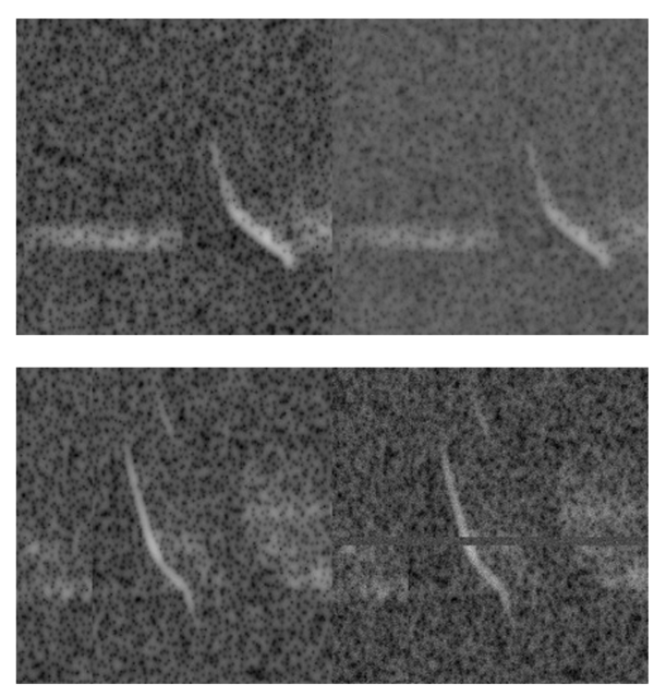
- A custom `SpectrogramDualView` class built on `imgaug` for spectrogram-aware augmentations. Image augmentations are used to generate variations of a test image that should map to a similar encoded representation. Standard image augmentations (color jitter, ImageNet-style crops) don't fit the time progression in a spectrogram.`SpectrogramDualView` produces views needed for learning while respecting the semantics of a spectrogram. It exposes a single `overall strength` knob plus a few targeted probabilities so we can explore augmentation intensities without hand-tuning every operator. The augmentation intensity settings and crop-based performance optimizations were added by USGS for the NABat bioacoustics use case.
Further details can be shared upon request.
6. Learning Data Pipeline / Compute Environment and Training Bottlenecks
Training was completed over multiple epochs. First, a data loader pulls precomputed spectrograms from Caldera, performs augmentations, and loads 224x224 pixel image patches onto the GPU. Training was then orchestrated using Slurm and standard GPU enabled PyTorch runners on the USGS Hovenweep cluster (Falgout J. et al. 2026). While a seemingly straightforward process, there were several challenges in this learning pipeline that required further engineering effort.
At first, training was limited by the speed at which the small files were being read from Caldera into the GPU node memory by the data loaders (I/O bound) this was particularly challenging since the individual images and noise files are relatively small. Hovenweep has limited high speed storage, and our datasets were too large to fit on a GPU node NVME drive. This led to an initial training rate of 0.17it/s which would lead to a total runtime of approximately two months to complete 100 epochs. To improve I/O performance we created WebDataset shards from the spectrograms. Each shard has a configurable size (set to 2GB in our case), which allows us to better saturate the interconnect between the storage and GPU nodes. After we adopted WebDatasets for training, the next bottleneck became CPU node performance on both memory and processor. As the shards were loaded and expanded in memory, the full spectrograms were augmented and then the portion that did not get selected for the patch was discarded. To best use the available hardware, we then pre-cropped the spectrograms. The processor heavy augmentations were now run only on the critical areas of the spectrogram, and the entire image did not need to be loaded into memory. Additionally, we precomputed 224x224 pixel patches from noise files and loaded a configurable number into memory (10,000 for initial experiments). Other optimizations included converting the image depth to an 8 bit integer from 32 bits to save memory on the GPU and extensively tuning the number of data loaders and batch size. These performance improvements led to an eight-fold improvement in training speed.
7. Training Metrics and Evaluation
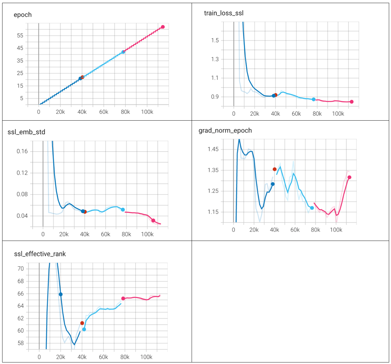
To measure the progress of training campaigns, we began by focusing primarily on training speed and the SSL loss metric. We are using a standard cross entropy loss metric for MoCo which calculates the similarity between image augmentations. As training progressed it became evident that additional metrics were needed to evaluate whether our choice of backbone, augmentation types and strengths, and learning rates were leading towards useful feature representations. We also wanted additional visibility into whether progress was being made towards improving downstream classifiers. This led us to using a linear probe every ten epochs to evaluate whether we were improving on a simple classification task. The linear probe runs every 20 epochs. We implemented Tensor board-style scalar logs that measure the following:
| Metric | Name | Description | Healthy behavior | Interpretation |
|---|---|---|---|---|
| ssl_emb_std | Embedding Standard Deviation | The average standard deviation of each embedding vector produced by the query encoder. | Embedding std should grow early (network explores space) then stabilize at a positive value (depending on feature scale) | < ~0.02: Danger: likely collapse or excessive normalization 0.05–0.2: Healthy for contrastive learning > 0.4: Unstable, too much contrast / augmentation |
| ssl_effective_rank | Effective rank | A fast approximation to the matrix rank using the entropy of eigenvalues of the feature covariance matrix. | Effective Rank tells you how many orthogonal directions the representation uses. Rank ~ 1 → collapse (catastrophic) Rank small → severe dimensional bottleneck Rank ~ 10–200 → healthy depending on architecture | With MoCo head output of 128 Healthy range: 20-80
|
| grad_norm | Gradient norm | The L2 norm of all gradients after backprop. |
Model collapse → gradients go to near‑zero Momentum discrepancies → oscillatory norms | Grows every epoch → explosion: Lower LR or reduce augment strength Drops near zero: Underfitting or collapse Oscillates mildly: Bad augment samples |
8. Model Experiments
For each experiment we define:
- Backbone: network being trained in the MoCo campaign
- Learning rate: which sets the step size for the optimizer
- Batch size: the number of image samples processed by the network in a single pass
- Num workers: sets how many CPU subprocesses are used in parallel to fetch, load, and preprocess data from the dataset before it is fed into the GPU
| Backbone | Learning rate | Batch size | Num Workers |
|---|---|---|---|
| MobileNet V2 | 0.01 | 256 | 16 |
Linear probe
The version numbers correspond with the linear probe campaign with version 0 beginning after the first 10 epochs of SSL training.
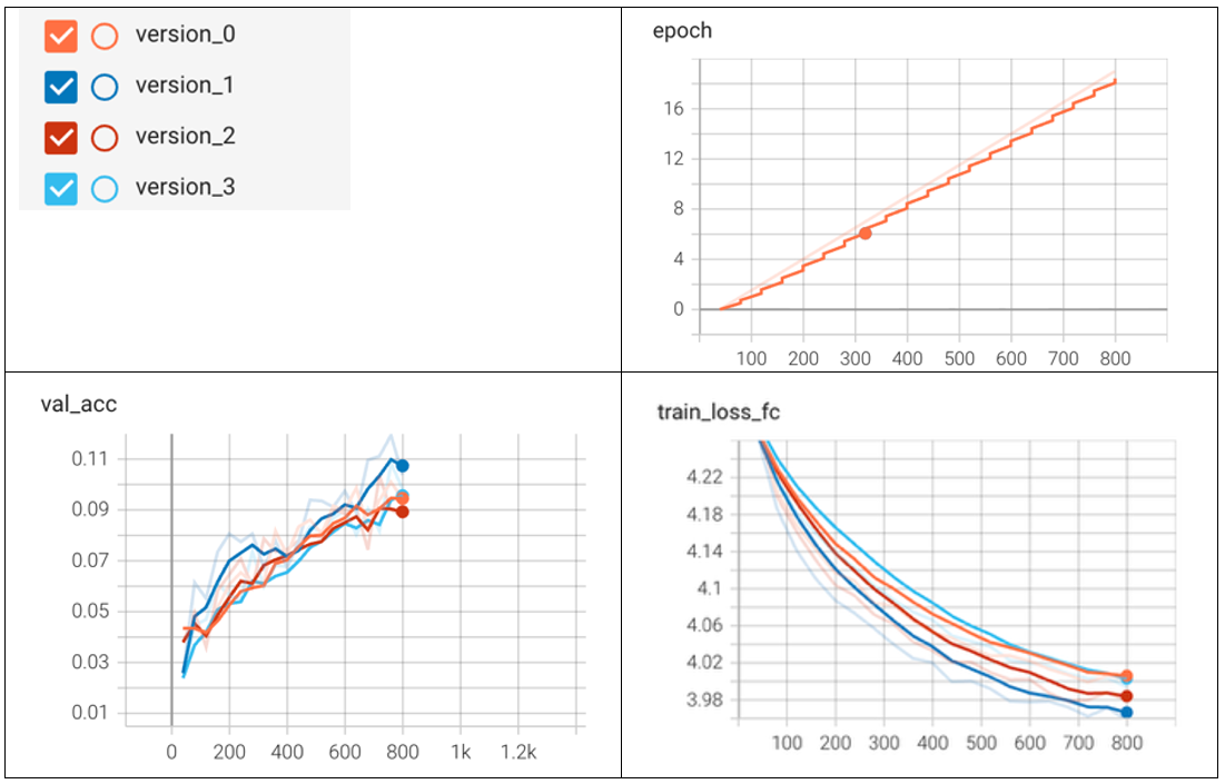
The training loss of the SSL backbone stabilized around 0.9 which is expected for the MobileNet backbone. The fact that the embedding standard deviation is low and the value accuracy of the linear probe has stalled after 20 epochs indicates that this version of the MobileNet backbone may be having a difficult time extracting meaningful features. Future experiments are expected to show improved embedding performance with a backbone with more trainable parameters, such as MobileNet v3 (Large) or an EfficientNet variant.
9. Future Work
We have built a training loop, datasets, and data loaders optimized for self-supervised learning on Hovenweep, a USGS cluster (Falgout J. et al. 2026). However, further experiments over the backbone variants identified above are still needed. Once we have identified the best configuration and augmentation strength for the initial bat classification task, we have a number of other use cases which will allow us to evaluate the generalizability of the resulting model. These use cases include processing data with acoustic noise from wind turbines, identifying bat call types (e.g., feeding buzzes and social calls), and classifiers that are specialized to a specific geographic region.
10. References
Bradley J Udell, Bethany R Straw, Tina Cheng, Kyle D Enns, Winfred Frick, Benjamin Gotthold, Kathryn M Irvine, Cori Lausen, Susan Loeb, Jonathan Reichard, Thomas Rodhouse, Dane A Smith, Christian Stratton, Wayne E Thogmartin, Ashton M. Wiens, Brian E Reichert. 2022. Status and Trends of North American Bats Summer Occupancy Analysis 2010-2019 Data Release. 10.5066/P92JGACB
Falgout, Jeff T, Janice Gordon, Lopaka Lee, Brad Williams, Accessed 2026, USGS Advanced Research Computing, USGS Hovenweep Supercomputer: U.S. Geological Survey, https://doi.org/10.5066/P927BI7R
Gotthold, B., Khalighifar, A., Straw, B.R., and Reichert, B.E., 2022, Training dataset for NABat Machine Learning V1.0: U.S. Geological Survey data release, https://doi.org/10.5066/P969TX8F.
Gotthold, B.S., Khalighifar, A., Chabarek, J., Straw, B.R., Reichert, B.E., 2024, North American Bat Monitoring Program: NABat Acoustic ML, (version 2.0.0): U.S. Geological Survey software release, https://doi.org/10.5066/P1QBMNSF
Kaiming He, Haoqi Fan, Yuxin Wu, Saining Xie, Ross Girshick. 2020. Momentum Contrast for Unsupervised Visual Representation Learning.
https://doi.org/10.48550/arXiv.1911.05722
Khalighifar, A., Gotthold, B. S., Adams, E., Barnett, J., Beard, L. O., Britzke, E. R., Burger, P. A., Chase, K., Cordes, Z., Cryan, P. M., Ferrall, E., Fill, C. T., Gibson, S. E., Haulton, G. S., Irvine, K. M., Katz, L. S., Kendall, W. L., Long, C. A., Mac Aodha, O. … Reichert, B. E. (2022). NABat ML: Utilizing deep learning to enable crowdsourced development of automated, scalable solutions for documenting North American bat populations. Journal of Applied Ecology, 59, 2849–2862. https://doi.org/10.1111/1365-2664.14280
Kitware Inc. https://www.kitware.com/
Jonathan D.; Irvine, Kathryn M.; Ingersoll, Thomas E.; Coleman, Jeremy T.H.; Thogmartin, Wayne E.; Sauer, John R.; Francis, Charles M.; Bayless, Mylea L.; Stanley, Thomas R.; Johnson, Douglas H. 2015. A plan for the North American Bat Monitoring Program (NABat). Gen. Tech. Rep. SRS-208. Asheville, NC: U.S. Department of Agriculture Forest Service, Southern Research Station. 100 p.
Reichert, B., and Lausen, C., Loeb, S., Weller, T., Allen, R., Britzke, E., Hohoff, T., Siemers, J., Burkholder, B., Herzog, C., and Verant, M., 2018, A Guide to processing bat acoustic data for the North American Bat Monitoring Program (NABat): U.S. Geological Survey Open-File Report 2018–1068, 33 p., https://doi.org/10.3133/ofr20181068.
Schwinger R., Vali Zadeh P., Rauch L., Kurz M., Hauschild T., Lapp S., Tomforde S., 2026, Foundation models for bioacoustics – A comparative review, Ecological Informatics, Volume 96, https://doi.org/10.1016/j.ecoinf.2026.103765.
Related

North American Bat Monitoring Program (NABat)
Related