
Models of Mercury in Fish
Environmental scientists and fisheries managers face formidable challenges in their efforts to better understand how mercury (Hg) is dispersed in the environment and to protect the public from exposure to methyl-mercury through the consumption of fish.
However, important spatial and temporal trends in the distribution of mercury are often obscured by natural variations between different fish species, sizes, and sample types. Futhermore, collecting enough samples of each fish species to achieve accurate assessments using current methods is often prohibitively expensive.
A statistical model has been developed which promises to overcome these challenges. The model improves analysts' ability to distinguish trends by factoring out the effects of variations between different species, sizes, and sample types of fish. Modeled data can be normalized to a large number of different species, length, and sample cuts. In this way, data from a single sample can be used to estimate mercury concentrations in many fish with very different characteristics, dramatically lowering sampling costs without decreasing accuracy.

By accounting for differences in mercury concentrations due to differing species, sizes, and sample types, the model allows data from samples with different characteristics to be analyzed together. In this way, data can be 1) normalized to a specific species, length, and sample type for assessing spatial and temporal trends, or 2) extrapolated to multiple species, lengths and sample types for preparation of fish consumption advisories.
This model uses a statistical method to:
- Measure the average proportional variation between different sample types collected within each sampling event ('event' refers to a specific site and time);
- Factor out the fish-Hg concentration variation attributable to the characteristics of the samples collected during the sampling event in order to determine the relative difference in fish-Hg concentrations observed at each sampling event; and
- Predict or map variations in fish-Hg concentrations by estimating fish-Hg concentrations for a consistent sample type (i.e. same species, portion sampled and fish length) across all sampling events.
Benefits of the Model
- Enhanced Analysis of Spatial and Temporal Trends - By factoring out natural differences in Hg concentration due to differences in fish species, length, and sample type, the model makes it much easier to spot significant spatial or temporal trends in the data.
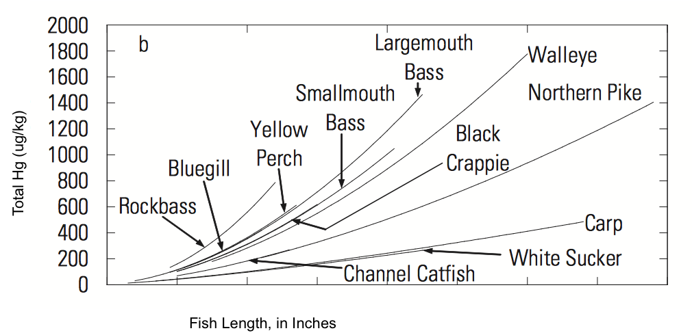
- Cost Effectiveness - Another important benefit of the model is the potential to improve monitoring program efficiency (cost per unit information generated). It should not be necessary to collect and analyze fish of all lengths in order to determine whether the largest fish are safe to eat. For example, if edible fish of a given species occur in lengths ranging from 8 to 25 inches but a sample includes only a 19-inch specimen and a 23-inch specimen, the model will allow mercury concentrations to be inferred for smaller fish. Since fewer samples are needed to produce comprehensive fish consumption advisories, analytical costs (costs associated with the chemical analysis of fish) can lowered substantially. In this way, program dollars can be stretched to produce much more information.