NHD Watershed Tool

This document describes how to collect and preprocess the support data layers. This document also describes the reasons for preprocessing, the appropriate data layers to use for preprocessing, and the functionality of the watershed tool. 

Table of Contents

• Watershed Tool Development
  • Figure 1
  • Figure 2
• Instructions
  • Preprocessing the NHD
    • Figure 3
  • Preprocessing the NED and watershed boundaries
  • Merging 10-meter DEMs with NED
  • Additional steps for the catchment data layer
  • Loading data into the NHD WATershed SUPport (WATSUP) data layers workspace
• Preprocessing programs and files
  • agree.aml
  • nedprocessing.aml
  • openme.txt
  • metadata document
  • runtopo.aml
• References Cited

_____________________________________________________________________________________________________

Watershed Tool Development

NHD Watershed is an enhancement to a watershed tool that was initially developed for the State of Massachusetts by MassGIS and the U.S. Geological Survey (archived by MassGIS). The tool was developed for watershed analysis, including the WEB application named STREAMSTATS (Ries and others, 2000), using data layers unique to the State of Massachusetts and thus was not immediately transferable to data layers available nationally. The processing described in this document enhances the tools developed for Massachusetts by integrating the functionality of the watershed tool in the NHD ArcView Toolkit with spatial data and related databases that cover (or are planned to cover) the continental United States. 

Preparing to use the NHD Watershed tool, as was the case with the Massachusetts tool, is based on modifying 3 spatial datasets: surface-water hydrography, land-surface elevation, and basin boundaries. Each of these data layers was modified to work in conjunction with the watershed tool and each other. Data layers corresponding to those used by Massachusetts are in various stages of development for use at the national level. 

At the national level, surface-water hydrography at 1:100,000-scale has been developed with a centerline network from USGS DLG data. This data layer has been attributed with EPA river reach codes and is now available as the National Hydrography Dataset (NHD). In addition, a number of states are developing 1:24,000-scale centerline hydrography data layers that conform to NHD standards. It is recommended that 1:24,000-scale NHD be used (as opposed to 1:100,000-scale NHD) for the preprocessing steps described in this document (a single source and scale (1:24,000 USGS topographic quadrangles) for all 3 input data layers is an important aspect of the capacity for these steps to work) . The NHD ArcView Toolkit watershed tool works only with centerline networks developed in the NHD. 

The land-surface elevation data has been developed nation-wide as the National Elevation Dataset (NED). The NED data used by the watershed tool is modified to create a grid with greatly exaggerated stream channels to resolve problematic watershed delineations, including watersheds delineated from river confluences and watersheds in large flat sinuous areas (the 'canyonized' stream channels exaggerate the vertical difference of the elevation values in NED for use in determining slope and other watershed characteristics). The approach provides a precise link between the vector NHD and raster NED data on stream channels, allowing for accurate watershed delineation. 

The basin boundaries data layer was developed in Massachusetts by digitizing 2,100 basins from boundaries scribed manually on Mylar quadrangle overlays. These Massachusetts basins vary in size, but generally are comparable to 14-digit hydrologic unit (HUC) basins. A number of states have digitized basin boundaries at similar densities. At the national level, a less dense 12-digit HUC basin boundary data layer is being developed by USDA's Natural Resources Conservation Service (NRCS) and USGS as the Watershed Boundary Data-layer (WBD), but is not yet available for most of the country (as of 4/2002). The boundaries are used in the preprocessing to exaggerate the height of NED data where the two data layers overlap (along the ridge lines). Use of these pre-existing basin boundaries, rather than delineating the basin entirely with NED, takes advantage of previous work, maintains consistency with pre-existing delineations, and ensures that the delineation is accurate in headwater areas. For the procedures discussed in this document, it is recommended that the data layers are preprocessed with as dense a basin boundary dataset as is available, as long as the dataset is accurate when draped on a 1:24,000-scale topographic map and horizontally accurate with 1:24,000-scale NHD in areas where the two datasets overlap. 

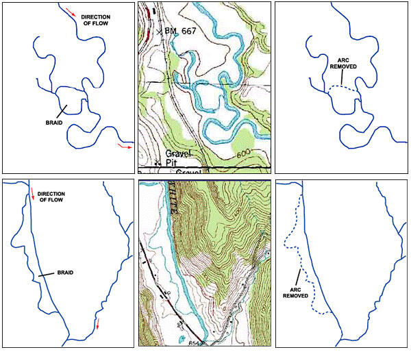
Preprocessing of the NHD is performed by first making a 'line' data layer of the NHD.RATRCH reach table from the selected NHD data layer (see the instructions below for step-by-step details). The new line data layer is then edited to remove arc segments on a case-by-case basis with the goal of eliminating braided networks (optionally, the braids could be left in with the caveat of unpredictable watershed results when selecting points on the network in braids). This procedure was completed for a pilot 8-digit HUC (NHD is tiled using the 8-digit HUC) by draping a Digital Raster Graphic (DRG) behind the NHD data layer and, for each braided network, determining where the least amount of flow was likely to occur. Once this determination was made the arc representing that flow was deleted from the network. Figure 1 diagrams this procedure in several areas. NOTE: the resulting data layer (see under the instructions: 'Preprocessing the NHD') is a by-product of NHD. The NHD itself is not edited. The results simply affect locations from which users can delineate watersheds on the NHD. The majority of locations on the NHD from which users will be able to delineate watersheds will remain intact. Finally, it is helpful to know how NHD determines flow before removing an arc. One way to do this is to use 'NHD Navigate' in the NHD ArcView Toolkit on each of the arcs that make up the braid. There may be occasions where the flow is incorrect. This will affect watershed delineation because NHD Watershed depends on NHD Navigate working correctly. If flow appears incorrect in these areas this would be an opportunity to correct the flow. If you are willing to make this correction and share the update with USGS, please contact USGS National Hydrography Support at nhd@usgs.gov for details. 

back to Table of Contents

Sources/Usage: Public Domain. View Media Details

The resulting data layer is comprised of a purely dendritic network. If this editing is not performed prior to modifying the NED data, watershed delineation will be inconsistent for any point delineated inside a braid (it may delineate correctly or delineate a small sub-watershed that does not reflect user intent). The developers of the watershed tool recognize that this editing step may be difficult to perform in some areas, particularly areas where complex networks (i.e. pipes/canals) have redirected flow. In these areas, it may be necessary to leave the braids as is and document the problems inherent with delineating local watersheds. 

The first step in preprocessing the NED is to 'clip' it to a 4000 meter buffer area around the selected 8-digit HUC. The 'clipped' raster grid is then converted into a point-data layer, and along with the dendritic stream network, is processed in ArcInfo (Environmental Systems Research Institute Inc., 1997) using the TOPOGRID command (TOPOGRID is an interpolation method specifically designed for the creation of hydrologically-correct digital elevation models (DEMs) from elevation and stream data layers). The output grid is then processed using agree.aml, whereby the dendritic NHD network is 'burned' into the elevation dataset. The result is a grid that is horizontally precise to the NHD data layer. A fill process is then performed on this output grid, followed by flow direction and flow accumulation functions, which create grids used by the NHD ArcView Toolkit watershed tool. 

Preprocessing of the basin boundary data layer is performed by first converting the boundary into a raster grid. After preprocessing the NED data layer, the grid cells that overlay the basin boundary lines are given an exaggerated value of 50 meters greater than the default elevation values at these locations. The effect is to force the on-the-fly watershed delineation to recognize the location of pre-existing basin boundaries. 

The final step in preprocessing is the creation of the catchment data layer (the surface area contributing drainage directly to a given reach). This data layer consists of one local drainage catchment for each NHD reach. The catchment data layer is created using the WATERSHED function in ArcInfo Grid. The WATERSHED function takes as input, the final flow direction grid (output from the NED preprocessing steps), and the raster grid representation of the NHD dendritic network. Each catchment is attributed with a corresponding reach code for a one to one relationship to NHD reach codes. 

Watershed delineation is performed in the watershed tool as follows. A point is selected on the centerline network. The tool then identifies and accumulates all upstream reaches and catchments in the watershed upstream of this point. Next, the selection point isolates the singular catchment that overlaps the point. The modified NED data is used to delineate a sub-watershed boundary within the isolated catchment from the selected point on the network. The NED derived sub-watershed boundary is then merged with the upstream catchments and internal boundaries are dissolved, resulting in a new watershed for the selected point on the network. In the NHD ArcView Toolkit, the newly delineated watershed is then attributed with identification characteristics, including reach code, distance along the reach where the point was delineated, and watershed area. Figure 2 diagrams these steps.

back to Table of Contents

Sources/Usage: Public Domain. View Media Details

The watershed boundaries determined from a selected point on a 1:24,000 scale stream reach are more accurately defined than a watershed boundary determined from a position on a 1:100,000 scale stream. This is because 1:24,000 hydrography is in better spatial agreement to the NED than the 1:100,000 scale NHD (NED and 24K NHD are typically derived from the same base map), especially near stream channels. Also, stream density at 1:24,000 is more appropriate for many applications of the watershed tools such as determining low flows of small streams and for regional planning applications. Thus, watershed delineation functionality of the watershed tools ideally would use 1:24,000 scale data. 

Below is a specific set of instructions for preprocessing the data layers used by the NHD ArcView Toolkit watershed tool. Any deviation from this approach could cause inaccuracies in watershed delineation that may not be traceable by the development team. 
 

back to Table of Contents

Instructions

Preprocessing the spatial data is described here using 'classic' workstation ArcInfo. Users may decide to replace some (or all) of these editing steps with steps in other software packages they may be more comfortable using. For example, NHD preprocessing can be easily replicated in ArcMap. In order to preprocess data using the steps below, the user will need to have workstation ArcInfo 8xx (or higher), its extension, Grid. 

It typically takes an experienced user 6-10 hours to step through these preprocessing steps. Variables to this time estimate include HUC size, computer resources (speed), database organization skills, and an initial learning curve. 

Preprocessing should not be performed in Geographic Projection (decimal degrees, or otherwise known as the "flat-earth projection"). Measurements like distance, angle, and area are completely invalid because the distances in x are different from the distances in y. Since analysis will be performed in the preprocessing steps and subsequent use of the data for applications, project your data layers to a projection of choice before using these editing steps. 

Keep in mind that NHD Watershed runs in ArcView 3.2. It also relies on the user having the ArcView 3x Spatial Analyst extension (there is an option for whole reach delineation (and not point along the reach) that does not require the user to have Spatial Analyst).

When reading the instructions:

• All ArcInfo commands are in capital letters: i.e. 'BUILD'.
   
• Comments that follow an ArcInfo command line are proceeded with a '/*': i.e. BUILD step6_cov poly /* check to see if any polygons still exist in the coverage.
   
• It is recommended that the coverage and grid names below (i.e. 'step4_cov') be used when stepping through the procedure. Some coverage and grid names are hard coded into the 'nedprocessing' aml, and several are referenced in subsequent steps.

back to Table of Contents

Preprocessing the NHD

1. Acquire the NHD workspace of interest from the NHD Web Site.
2. Copy the NHD data layer (named 'nhd') out of the NHD workspace and into a working workspace.
3. Project this new data layer into a projection of choice. Since all the data layers used in the preprocessing will be modified with a number ArcInfo commands, it is necessary to project them out of geographic coordinates (see intro to instructions above). Also, since DRGs will be used as a base for several editing procedures (and possibly in the NHD ArcView Toolkit as an image catalog), it would be ideal to project this data layer and the others to the projection of the DRGs you are using. Processed data layers can ultimately be kept in the projection of choice, since the NHD ArcView Toolkit allows users to work in any projection. Keep in mind that DRGs are often in 1927 datum. Make sure all projection and datum parameters match before editing.
4. Build the output of step 3 as a 'polygon' data layer: Arc: BUILD step4_cov poly
5. Run 'ROUTEARC' on the output from step 4: Arc: ROUTEARC step4_cov rch step5_cov.
6. Clean the output from step 5 as a 'line' data layer: Arc: CLEAN step5_cov step6_cov .5 .004 line.
7. In Arcedit, remove all isolated arcs in step6_cov that are not connected to any network that flows out of the 8-digit HUC. In most 8-digit HUCs, one river exits. Most coastal HUCs, however, have multiple rivers exiting. Isolated arcs need to be removed in order to avoid creating deep sinks during the NED preprocessing steps. One way to do this is to select at least one arc on each network (try selecting a number of arcs on various parts of the network) and run the 'aselect' command over and over until no new arcs are added to the selected set. Next, run the 'nselect' command, which flops the selected set to be all un-networked arcs. 'Delete' these arcs.
8. Select all remaining arcs and 'flip' them. This is needed because the NHD reach table (the table converted to a coverage for these preprocessing steps) has arcs facing upstream. For these procedures, arcs need to be facing downstream.
9. Extend the exit centerline arc(s) to at least 50 meters beyond the edge of the 8-digit HUC boundary (this may already be the case) while keeping in line with the centerline of the downstream HUC. The 50-meter buffer zone around the 8-digit HUC is maintained through the NED preprocessing steps. This boundary should ultimately coincide with the data/no-data boundary of all final output grids (see step 13 of 'Preprocessing the NED and watershed boundaries). This can be accomplished by adding additional vertexes to the line or moving the end vertex (node) as needed, however, the horizontal alignment of the existing centerline data must remain unchanged. By extending the exit centerline arc(s), you will avoid the creation of a permanent sink for the network or any attempt by the preprocessing to fill it. If you are running these procedures on a coastal 8-digit HUC, which has multiple NHD mouth points, it may be helpful to add and connect lines out into the ocean (to keep track of them). Finally, if the 8-digit HUC is downstream of other 8-digit HUCs, include the exit stream(s) of the upstream 8-digit HUC(s).  (See Figure 3)
10. Save step6_cov. Quit out of Arcedit. Build as a line data layer. 
11. Make a copy of step6_cov: Arc: COPY step6_cov step6_bak. Build step6_bak as a poly data layer: Arc: BUILD step6_bak poly.
12. In Arcedit, edit step6_cov. Using step6_bak as a background data layer (BACKENVIRONMENT poly fill), and Digital Raster Graphic images of the USGS quadrangles (DRGs), step through each polygon and determine which arc to remove so as to eliminate the braid. Read through the paragraph above 'Preprocessing of the NHD data layer is performed as follows', and the accompanying figure 1 for more details. When removing arcs, it is helpful to have arc arrows turned on to avoid any remaining arcs from pointing upstream (this has an adverse affect on TOPOGRID).
13. Save step6_cov. Quit out of Arcedit.
14. Arc: BUILD step6_cov poly /* Check to see if any polygons still exist in the coverage. If so, repeat steps 11-13, until building the coverage as a poly data layer produces zero polygons (after completing this, repeat step 7 to see if any arcs were left unconnected to the network during this editing procedure. If so, delete the unconnected arcs).
15. Arc: BUILD step6_cov; Arc: DROPFEATURES step6_cov poly; RENAME step6_cov nhdrch.

back to Table of Contents

Sources/Usage: Public Domain. View Media Details

back to Table of Contents

Preprocessing the NED and watershed boundaries

As an initial quality control step, you may want to review the accuracy of your watershed boundaries (particularly if they have not yet been approved as part of the Watershed Boundary Data-layer (WBD). The areas of greatest concern would be at NHD confluences (i.e. where boundaries are delineated to confluences, do they cross the stream at or near the true confluence point? Do they cross over the streams at inappropriate locations?) and headwaters (do NHD headwaters cross over your watershed boundaries? If so this would most likely reflect an inaccurately delineated watershed boundary). Minor edits may need to be made to the boundaries. However, if wholesale changes are needed, there may need to be a reassessment of whether or not to use the watershed boundaries. The preprocessing steps to be followed are:

1. Acquire the NED data in the area represented by the 8-digit HUC of interest. This acquisition would include NED data within a 4000-meter buffer area around the 8-digit HUC. If it is necessary to merge tiles of NED data, do this before projecting (see step 2 'Merging 10-meter DEMs with NED'). ** IMPORTANT: Re-sampled 10-meter DEMs can be used in place of NED data, where they are available. Determine the availability of 10-meter DEMs. To use 10-meter DEMs in place of NED where 10-meter DEMs exist for the entire 8-digit HUC, follow these steps. However, for areas where 10-meter DEMs exist for only portions of the HUC, see the section immediately below 'Merging 10-meter DEMs with NED'.
2. Project the NED data to your projection of choice (see 'Preprocessing the NHD' step 3). When projecting NED data, use bilinear interpolation, or, if projecting in Grid, make sure that SETCELL is set to the default (maxof) and that you specify the output cell size (�30� if working with 30-meter NED data) as an argument at the command line. Also, set the x_register and y_register to 0, 0. This setting will make it easier to align the output raster origin cell (lower left cell) with subsequent elevation derivative grids (i.e. the flow direction and flow accumulation grids). The output grid will be named 'ned_g' for these instructions.
3. ned_gcm = ned_g * 100 /* Convert the elevation units (zunits) of the NED grid ('ned_g') from meters to centimeters because the data will be truncated when it is converted to an integer grid during preprocessing (the z values may already be in centimeters: check the metadata).
4. Create two buffer data layers using the 8-digit HUC data layer as input. The first buffer area will be a 4000-meter buffer (Arc: BUFFER huc_cov buff_4000 # # 4000 2 poly). This buffer area will be used as the clipping area for TOPOGRID interpolation of the NED. In order for accurate interpolation of the 8-digit HUC ridgelines, TOPOGRID needs the ability to compute not only what areas flow into the HUC, but also what areas flow out from the HUC ridgeline. The second buffer area will be a 50-meter buffer (Arc: BUFFER huc_cov buff_50 # # 50 2 poly). This buffer data-layer will be used as input for the TOPOGRID sub-command 'BOUNDARY'. An important point to remember is that it may be necessary to tile the basin into 2 or more parts prior to this step, depending on computer resources. TOPOGRID, particularly as used here, can create a high demand on your computer system. Virtual memory needs to be monitored and reset if resources are available. It may help to skip ahead to the TOPOGRID step and bomb out of the process intentionally to optimize the computer resource adjustments and determine the amount of basin tiling that may be necessary. If the basin needs to be tiled into 2 or more parts, it is recommended to do so along sub-basin divides, rather than along straight-line rectangular quadrangle boundaries or other straight-line rectangular tiles. If the HUC is tiled, set up sub-directories and run steps 4 thru 11 in each of these sub-directories (the resulting datasets in each sub-directory will overlap ~ 4000 meters if the procedures are followed correctly).
5. Grid: SETWINDOW buff_4000 ned_gcm.
6. Grid: buff_4000g = POLYGRID (buff_4000,#,#,#,10) /* converts the buffered basin boundary to a grid.
7. Grid: SETMASK buff_4000g.
8. Grid: ned_clip = ned_gcm.
9. Arc: DESCRIBE ned_clip /* retain the 'Xmin', 'Ymin', 'Xmax', and 'Ymax' values for the 'xyzlimits' subcommand in TOPOGRID (see step 11e below).
10. Arc: VIP ned_clip ned_pnts 85 /* converts the NED raster grid data layer to a point data layer for input into TOPOGRID. Remove values '0' and less than '0' from the point coverage (exceptions: Death Valley CA, New Orleans, and possibly other areas with elevations below sea level).
11. Arc: TOPOGRID topogr_gr 10 /* cell size is re-sampled to 10 meters. An aml runtopo.aml is attached to assist the user through this step.
    1. Topogrid: BOUNDARY buff_50.
    2. Topogrid: ENFORCE on.
    3. Topogrid: POINT ned_pnts spot.
    4. Topogrid: STREAM nhdrch /* if the basin is tiled, this data layer should first be clipped into the tiled 'buff_50' data layer.
    5. Topogrid: XYZLIMITS xmin ymin xmax ymax /* These values are calculated by taking the values from step 9 (above), adding 5 meters to the 'Xmin' and 'Ymin' values and subtracting 5 meters from the 'Xmax' and 'Ymax' values, and rounding the results to the nearest number divisible by 10 (see the on-line help menu for 'TOPOGRID' for more details on the 'XYZLIMITS' subcommand.
    6. Topogrid: END.
12. If the basin was tiled, merge the 'topogr_gr' grids back together in the upper level workspace. Example: Grid: topogr_gr = MERGE (sub1_dir/topogr_gr, sub2_dir/topogr_gr, sub3_dir/topogr_gr).
13. Double check to make sure that the 'nhdrch' exit centerline extends beyond the data/no-data boundary of the 'topogr_gr' grid (see step 9 'Preprocessing the NHD' and figure 2).
14. Run the program nedprocessing.aml on the merged 'topogr_gr'. Four data layers must exist in the workspace for this program to run correctly: the preprocessed NHD reach data layer ('nhdrch'); the TOPOGRID results data layer ('topogr_gr'); the 8-digit HUC data layer ('huc8'); and the sub-basins data layer, which can be HUC12 or better ('subbas_24'). This processing does a number of things, including the 'burning' in of stream reaches using agree.aml and exaggerating the ridge lines where elevation cells overlap lines from the 'subbas_24' data layer. The aml (nedprocessing.aml) also creates the final flow direction ('dir2'), flow accumulation ('accum2') and catchment data layers ('shed_cov'), which are all used by the watershed tool. For users of ArcHydro, a slightly updated version of nedprocessing.aml exists. Please contact Pete Steeves for a copy (psteeves@usgs.gov).

back to Table of Contents

Merging 10-meter DEMs with NED

Re-sampled 10-meter DEMs can be used in place of NED in areas where the data is available. As is the case with the original 30-meter DEM data layer, 10-meter DEMs are processed by 7 � minute topographic quadrangle, therefore, 10 meter DEMs may not be complete for an entire HUC. The steps below outline how to piece the 10-meter DEM data in with NED data.

1. Follow steps 1-10 above ('Preprocessing the NED and watershed boundaries') for the NED data.
2. Grid: dem10_all = MERGE (dem10_1, dem10_2, �, dem10_X) /* merge all available 10-meter DEMs.
3. Project the merged 'dem10_all' to the projection of choice (see step 2 'Preprocessing the NED and watershed boundaries'). The output grid will be named 'dem10_allp' for these instructions.
4. dem10_allc = dem10_allp * 100 /* Convert the Zunits of the 10-meter DEM grid (dem10_allp) from meters to centimeters: because the data will be truncated when it is converted to an integer grid during preprocessing.
5. VIP dem10_allc dem10_pnts 35 /* converts the 10-meter DEM grid to a point coverage /* also, if the basin needs to be tiled (see step 4 'Preprocessing the NED and watershed boundaries'), CLIP the dem10_pnts into the tiled area and put the resulting clipped point data layer into the appropriate sub-directory prior to running TOPOGRID.
6. Grid: maskcov = GRIDPOLY (setnull(isnull(dem10_all),1)) /* creates a mask coverage of all areas with 10-meter DEMs.
7. Arc: ERASE ned_pnts maskcov ned_pnts_e point /* erase all NED points that overlay 10-meter DEM points.
8. Arc: TOPOGRID topogr_gr 10. /* An aml runtopo.aml is attached to assist the user through this step.
   1. Topogrid: BOUNDARY buff_50.
   2. Topogrid: ENFORCE on.
   3. Topogrid: POINT ned_pnts_e spot.
   4. Topogrid: POINT dem10_pnts spot.
   5. Topogrid: STREAM nhdrch /* if the basin is tiled, this data layer should first be clipped into the tiled 'buff_50' data layer.
   6. Topogrid: XYZLIMITS xmin ymin xmax ymax /* These values are calculated by taking the values from step 9 ('Preprocessing the NED and watershed boundaries'), adding 5 meters to the 'Xmin' and 'Ymin' values and subtracting 5 meters from the 'Xmax' and 'Ymax' values, and rounding the results to the nearest numbers divisible by 10 (see the on-line help menu for 'TOPOGRID' for more details on the 'XYZLIMITS' subcommand).
   7. Topogrid: END.
9. Follow steps 12 and 14 above ('Preprocessing the NED and watershed boundaries').

back to Table of Contents

Additional steps for the catchment data layer

The reach code is needed as a permanent link between the NHD reaches and the catchment data layer. Since the reach code is a character item, it could not be used in the preprocessing steps described above. The 'com_id' item in NHD is temporarily used to establish the link. The steps here describe how to replace the 'com_id' item with the reach code item.

1. Arc: ADDITEM shed_cov.pat shed_cov.pat rch_code 14 14 c.
2. Arcplot: RELATE add.
   1. Relation name: comid.
   2. Table identifier: nhdrch.aat.
   3. Database name: INFO.
   4. INFO Item: grid-code.
   5. Relate column: com_id.
   6. Relate type: Linear.
   7. Relate Access: RW.
3. Arcplot: CALCULATE shed_cov poly rch_code = comid//rch_code.
4. Arc: DROPITEM shed_cov.pat shed_cov.pat grid-code.

back to Table of Contents

Loading data into the NHD WATershed SUPport (WATSUP) data layers workspace

1. Create an NHD WATershed SUPport (WATSUP) data layers workspace: prefix = 8-digit HUC code; suffix = '_ws' (ie 01080105_ws).
2. Three data layers get loaded into the WATSUP:
   1. Copy dir2 (created in the NED processing) into the new workspace and call it 'dir_grd'.
   2. Copy accum2 (created in the NED processing) into the new workspace and call it 'accum'.
   3. Copy shed_cov (created in the NED processing) into the new workspace.
3. Convert the data layer 'nhdrch' into a shapefile: Arc: ARCSHAPE nhdrch line dendrite. Copy the shapefile 'dendrite' into a WATSUP sub-directory called 'dendrite', along with the .dbf and .shx files.
4. Access the generic openme.txt  file and load it into the WATSUP workspace (the 'openme.txt' file is selected by the user with the menu option 'Select WS Tools Support Data Location' in the NHD ArcView Toolkit).
5. Access the WATSUP metadata document, modify to your specific processed CU, convert the modified document to HTML format, and load into the WATSUP workspace.
6. The data is now ready to use in the NHD ArcView Toolkit.

back to Table of Contents

References Cited

Environmental Systems Research Institute, Inc., 1996, Using ArcView GIS: Redlands, Calif., 350 p. 

Environmental Systems Research Institute, Inc., 1997, Advanced ArcInfo Volume 1 and 2: Redlands Calif. 

Ries, K.G., Steeves, P.A., Freeman, A., and Singh, R. 2000, Obtaining Streamflow Statistics for Massachusetts Streams on the World Wide Web: U.S. Geological Survey Fact Sheet 104-00.