
What's New? Weeks 5-8
Check this page each Tuesday for new things to explore!
Week 8: 5/5 Floods and Hurricanes

Did you know that the first week of May is National Hurricane Preparedness Week? Even if you don’t live in a coastal city, hurricanes are fun to study, and they have a lot in common with floods. Hurricanes, floods, and droughts are the costliest natural disasters. Both hurricanes and floods start to increase in the spring and are common through the summer and into early fall.
A flood is any relatively high streamflow that overtops the natural or artificial banks of a river and a hurricane is a strong, rotating storm with high winds (>64 mph) that is powered by warm ocean water (around 80 degrees F at the surface, or higher). While hurricane winds do a lot of damage, much of the destruction is caused by floods due to torrential rains and storm surge, which is ocean water that pushes toward the shore.
Floods
Grades 3-12: Streamgages and Water Levels
How much water is flowing in a river? Is the flow below, at, or above normal? How is stream flow measured?
Since 1889, the USGS has been measuring stream flow and water-related hazards, such as floods and hurricane storm surge, by using a network of more than 10,000 streamgages across the United States that provide important real-time data. The data from these streamgages are used to keep the public safe and to help emergency management experts make informed decisions.
Streamgages may just look like little houses on the outside, but they contain important equipment for measuring streams. Head on over to the USGS Water Science School to learn how a streamgage works.

Let’s take a look at streamgages across the US for a whole year. This animation shows a dot for each USGS streamgage, and the color changes with river level. Take a look at the scale, and then play the animation. You may want to watch it a few times.
- Are there times of year when flooding is more common?
- What are some causes of flooding?
- Are there places in the US that did not flood in 2018?
- Watch it again, and look just at one state. What do you see?
Water Watch:– Check out the real-time data near YOU. The Water Watch site has each USGS streamgage linked. You can select your state and then pick a single creek or river nearby, or explore any other place in the US that looks interesting today.
- Where is it flooding right now?
- Where is it drier than normal?
Click on any single dot – this tells you where the streamgage is and leads you to the data at that site.
- What is the closest streamgage to you?
- Look at the graph of gage level for the last week. Is your stream rising, falling, or staying the same?
- Write down the gage level, and then take a look again next time it rains. Do you see a difference?
In the spring of 2019, there was a week of heavy rain in the Midwest. This data visualization shows the rainfall, the rivers, and the USGS streamgages. Both the Mississippi and the Arkansas rivers had major flood events that spring, and this rainfall event was a major contributor.
Head back to Water Science School for some information about floods. Read the parts that most interest you. You may want to pay attention to the recurrence interval and 100-year flood because we are going to have some fun with that. Here is a poster about the 100-year flood.
Grades K-3: Drawing weather and storms
Draw yourself on a rainy day, maybe splashing in puddles, or watching a creek rise.
Hurricanes are storms that look like a spiral from above. Can you find something around you that looks like a spiral? Hint…spirals are common shapes in nature, perhaps you can find a snail or a fossil ammonite?
Grades 6-8: Size and Occurrence of floods
Scientists rank the size of floods by the probability, or likelihood, of a flood of that size happening. It is a matter of averages. If you could watch a river and measure its floods for 500 years, then the one biggest flood during that whole time would be a 500-year flood (once in 500 years). The much smaller flood-level that happened 500 times is known as the annual flood. What would you call a flood-level that happened 5 times in 500 years? (answer follows...)
Here is a classroom activity that you can do at home to chart the flooding probability of a river. You don’t need a group, but you do need 100 things that are the same and feel the same, but have different colors. You can use whatever you have around the house, such as pony beads, marbles, or dice. If you don’t have anything like that, cut out squares of colored paper, or mark 100 pennies with different colors of nail polish. You need five colors in the following ratio: A: 1 item, B: 2 items, C: 10 items, D: 20 items, E: 67 items. Have fun! (The answer above is a 100-year flood.)
Did you know that people have been recording flood levels for a really long time? Records in Egypt and China, for example, go back thousands of years. The oldest USGS streamgage was installed in 1889.
Grades 9-12
Read about 100-year floods and how we use data to determine flood designations.
Then, get ready to dig into some data yourself. This exercise leads you through the process of building a 100-year flood map for a community that you are interested in. You can use the Water Watch link above to choose a stream near you, or just use the one the exercise suggests. You’ll need to download 50 or more years of data, and do some calculations in a spreadsheet. Then, find the USGS topographic map of the site to plot your results. Share your results with us on Twitter @usgs_yes!
Perhaps you are interested in being a scientist one day. Here’s a video about how USGS hydrologists study floods and long-term streamflow data.
6-12th grade teachers: Here is a Flood Activity using remote sensing and Landsat imagery from AmericaView. Also, this is a downloadable slide presentation about how scientists do flood inundation mapping.

K-6: Make your own rain gauge! A rain gage is one simple tool you can use to measure precipitation from your own yard or porch. Here are a few examples of rain gauges.


All Ages: Make your own rain gauge in four easy steps

- Use scissors to carefully cut the top off of a lightweight plastic bottle.
- Add rocks or sand to the bottle so the wind won’t knock it over easily, then completely cover the rocks or sand with water, making sure that all the pore spaces are filled in. Place the top of the bottle at the top, upside down, to create a funnel. Secure with tape.
- Use a ruler to mark increments (in inches or centimeters) onto a piece of paper.
- Tape another color of paper or tape to mark the zero line at the top of the water in your bottle. Tape your measured increments paper to the bottle, completely covering the paper so it doesn’t get wet! Place your rain gage outside in an uncovered area on a rainy day. Compare with local weather reports to see how accurate your measurements were! Note: straighter-sided bottles will likely give more accurate measurements than bumpy bottles.
Some additional information about floods for those very interested
Floods on purpose? Why? Natural floods periodically provide sediment and nutrients to river banks. Rivers with dams, such as parts of the Colorado River in Arizona, no longer flood naturally, so the USGS and other partners including the Bureau of Reclamation studies experimental high-flow experiments and their effects on riparian (river edge) ecosystems and sediment distribution. Learn more about that research here.

Paleofloods

USGS scientists measure high-water marks from active storms, and also study floods in the past, known as paleofloods. See this example from paleofloods of the Tennessee River, this “oldie but goodie” 1976 publication about Glacial Lake Missoula and the Channeled Scablands of Eastern Washington, and a series of 2003 USGS inundation maps about these dramatic Pleistocene flooding events.
HURRICANES

This week (May 3-9) is National Hurricane Preparedness Week. Hurricane season in the northern hemisphere generally lasts from June-October when ocean surface temperatures are higher. Warm water drives hurricanes. The USGS works with the National Hurricane Center and other agencies to monitor hurricanes. One of the ways USGS field crews do this is by installing special sensors before, during, and after a hurricane.
Movie Time! Watch this video about how the USGS prepares for hurricanes. and this one on why studying coastal storms is so important. Finally, one on how we prepared for Hurricane Dorian, then we’ll look at those data.
Hurricane Dorian, the fourth named storm of 2019, was a massive Category 5 hurricane that did extensive damage in the Bahamas. Perhaps you remember seeing it on the news. As Dorian headed toward the US, USGS scientists set out a whole array of sensors to measure the storm surge along the Florida, Georgia, South and North Carolina coasts.
Grades 6-12: Take a look at the Hurricane Dorian Flood Event Viewer – Zoom in and click on any of the 'data diamonds' to see the data. The blue diamonds tell you how high the storm surge reached (in feet).
- Look at some storm surge levels on the coast and further inland. How high did the water get? If you were standing there, would it have been over your head?
- Look at the black triangles. These are USGS streamgages. Remember that some of the damage from hurricanes is from heavy rainfall. Click on some of those triangles. Does the water rise and then fall again in response to hurricane rains?
For more about Hurricane Dorian 2019, take a look at the USGS research site.
Grades 3-12: Before-and-After Images: Scientists learn a lot about natural processes by carefully looking at before-and-after images. You can sharpen your science-detective skills by making observations of these images before an after coastal storm events. Here are some tips:
- Focus on things that are lasting differences, like sand movement or trees being blown down.
- Ignore things that are not lasting, like clouds, the tide line, animals, or automobiles.
- Color changes to the plants could be damage from the event, or could be seasonal differences, so pay attention to the dates on the photos.

Compare these aerial photographs from before and after Hurricane Matthew (October 6-9, 2016). What differences do you see? Make a list of the changes you observe in the before-and after-images. If you lived in one of those houses facing the water, would you be worried about the next storm?
Now, let’s look at what a storm can do to the reefs and shallow marine environment. These images are taken from above, looking at the Florida Keys after Hurricane Irma (2017). In the left-hand images (before) the deep purple at the bottom of the image is deep water and the turquoise and bright blue are the shallows, coral reefs, sandy areas, and sea grasses. How does it look after? Do you see changes in the land?
To see other before-and-after images from Hurricane Matthew (2016), visit this page.
Grades 6-12: USGS has a citizen science project that lets you be the scientist and find and report differences in photos of the coast taken at different times. iCoast is your portal to being a USGS scientist for awhile. Check it out at: https://coastal.er.usgs.gov/icoast/ and make your contribution to science.
All ages: Watch this video by the St. Petersburg Coastal & Marine Science Center to learn more about coastal erosion and learn how to make your own coastal erosion model in your classroom or living room.
Build your own Storm Damage Model. You will need: a large tray, water, sand or dirt, model houses or other structures, and a fan.
Grades K-5: Download our Coastal Hazards Poster for elementary school. You can choose the colored version, or color it yourself. On the back are some hands-on activities to do at home.
Finally – here is a little animation on coastal inundation forecasting a storm surge for Madeira Beach, Florida, September 10–12, 2017.
Week 7: 4/28

This week, we’re highlighting amphibians. What is an Amphibian? Amphibians are vertebrates (animals with backbones - Phylum Chordata, Class Amphibia) that can live in a wide variety of habitats on land, water, or both (wetlands) ecosystems. Common examples of amphibians include: frogs, toads, newts, salamanders, many more – about 230 species in the continental United States alone!
Young amphibians (larvae) usually undergo a HUGE change (metamorphosis) from swimming as babies to land-living, air-breathing adults (gills to lungs, fins to feet). Amphibians also have unique skin and can use it to breathe or as a back-up to breathing or air exchange. Because they can inhabit so many places with different life stages and can exchange air and water with their skin, they are ecological-health indicators, which means that when something is wrong in the environment they are among the first vertebrates to disappear or show declines in health.
The USGS studies amphibians because changes in their abundance, or abnormalities in their life cycles or morphologies (shapes) often indicate that something is wrong in the environment before humans can see it or detect it (see one example about ecosystem health in this USGS Saving Salamanders story). The USGS Ecosystems Mission Area researches and monitors amphibians and many other kinds of fish and wildlife. Stay tuned for upcoming topics related to other Ecosystems topics.

Grades 6-12: Amphibian Research Monitoring Initiative
The USGS Amphibian Research and Monitoring Initiative (ARMI - link above) has branches across the country, and studies things like amphibian deformities, species ecology, the effects of climate change, invasive species, fire, and other impact on amphibians. Follow the link above to their website, and read about the things you are most interested in. Be sure to check out the photo page for some great shots of amphibians in the wild. You can download any of them.
Learn more about the North American Amphibian Monitoring Program here.
Did you know that Great Smoky Mountains National Park in Tennessee is known as the “Salamander Capital of the World?” Download USGS Circular 1258 Monitoring amphibians in Great Smoky Mountains National Park, here. Then take a look at another USGS Salamander Project with Patuxent’s Managing the Extinction Risk of the Shenandoah Salamander.

Grades K-2, plus all ages: coloring, dot-to-dot, and photo galleries
Frog Dot-to-Dot: https://www.usgs.gov/media/files/frog-connect-dots
Amphibian Image gallery: https://armi.usgs.gov/eyes-and-ears-of-ARMI.php
The Western Aquatic Research Center in CA has developed many fun and informative wildlife coloring sheets. We have compiled four of their amphibian friends (California Newt, American Bullfrog, American Toad, and Mountain Yellow Legged Frog) into an Amphibian Coloring Book that can be downloaded here.

All ages: Ribbit….Ribbit…Have you ever heard a chorus of frogs?
First, listen to a story about how and why USGS studies frog sounds with our Outstanding in the Field Podcast – Episode 4 – Amphibian Surveys Episode Call of the Frog
Next, listen to this chorus of evening frog calls here. Frogs can blend into their surroundings, making them hard to see. So, USGS researchers also rely on their sense of hearing to study frogs!
How well do you know your frog calls? You can test your frog-knowledge with the USGS Patuxent WIldlife Research Center's Frog Quizzes.

All Ages: How does a toad cross a road? Check out Toad Road for some fun, and safety, for toads. If you were a toad, would you want to travel this road?
Take a walk in your neighborhood and start a journal about amphibian activity in the water near you. It's springtime, do you see eggs, or tadpoles? Take a photo or better yet a video, note the date, and come back regularly to check. Let us know what changes you see! You can download a printable amphibian larvae (tadpoles and more) ID guide here.

Grades 9-12: Nonindigenous Aquatic Species (NAS) program - a Citizen Science Project
One of the projects at USGS in the Ecosystems Mission Area involving amphibians is the Nonindigenous Aquatic Species (NAS) database and citizen science project. NAS is an information resource or database about introduced aquatic species and is housed at the Wetland and Aquatic Research Center (WARC) in Gainesville, FL. The database is accessible by anyone and provides data, reports, maps, and general information about aquatic species that are not native to a habitat and referred to as non-native, invasive or nonindigenous from all over the U.S. The database was started because of the passage of the Nonindigenous Aquatic Nuisance Species Control and Prevention Act of 1990.
The law discusses aquatic nuisance species being introduced by ballast water vessels – what does that mean?
Why would ballast water have an influence on invasive species?
Which branch of government created the bill and brought it up for discussion and eventually passage?
Which state representative was responsible for the bill, why is that important?
Why does the USGS study nonindigenous species?
More than 6,500 nonindigenous species are established in the U.S. and they pose risks to native plants, animals, ecosystems and human and wildlife health. For example, the USGS is involved in the study and tracking of invasive zebra and quagga mussels as they invade and spread across North American especially in the Great Lakes and Upper Mississippi River basins. They have no natural predators in these aquatic areas, and they grow rapidly and clog up water, pipes, and water intake areas, which can cause water outages.
Go to the NAS database and search for Taxa Information for Amphibians.
How many Nonindigenous Amphibians are listed in the NAS database (hint: look for Species List of Nonindigenous Amphibians)?
Once you have found amphibians, look for the Data Queries option. You can Search by State for nonindigenous amphibians.
Look for your state – how many amphibians are listed as nonindigenous for your state?
Under More Info, click on the Point Map – look for how many observations of the nonindigenous amphibian(s) were collected in your state. How many were counted for each invasive amphibian?
Under More Info you can also find a species profile that will give you more information.
Where did this amphibian come from originally?
When was it first observed?
How was it introduced?
What has the impact on the ecosystem been due to its introduction?
Why might this amphibian be harmful to your locality?
How could you use this database’s information to conduct your own studies? How might you use this in your current online classroom?
Finally – how might you get involved in helping the USGS and other federal agencies track invasive amphibians? Go to the link Report a Sighting. If you have seen amphibians in your local wildlife area and you want to check on whether they are native or nonindigenous you can report a sighting. You can take a picture and upload it to the site, describe in detail where you saw it, when and any other information you can collect about the amphibian. Your observations will expand the ability of this databased to track and catalog invasive amphibians and help USGS scientists control invasive species.
Week 6: 4/21
This week is National Park Week! So, we’re featuring our Geology and Ecology of National Parks website. All kinds of adventures await you.

The USGS and The National Park Service, are both bureaus in The Department of Interior. We have been working together on various research and monitoring projects for over 100 years. Visit the park links below to learn about geologic processes, landforms, park ecology, and more!
The Youth & Education in Science (YES) team has been working (virtually) with college interns to update our Geology & Ecology of the National Parks website and to, where possible, add more to our pages about our various USGS-NPS collaborative projects. We are grateful to our hard-working interns for their contribution. You can explore anywhere on our Geology and Ecology of National Parks website, but the parks listed below have recently been updated, so they are a good place to start.
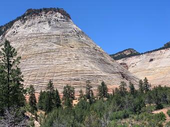
Sand and More Sand! These parks feature sand and other things. You can download, color, and build several different 3D paper Sand Dune Models. You’ll learn how sand dunes form and the various shapes they take. Many national parks have active sand dunes, and some in the desert Southwest (Zion, Capitol Reef, Canyonlands, etc.) have phenomenal examples of ancient sand dunes preserved in Mesozoic sandstones!

Sand Dune Models - best for Grades 6-12
Cape Cod National Seashore (Massachusetts)
Caves and Hot Springs: Water can form some pretty spectacular features. Check out these caves in Kentucky and South Dakota, and hot-water springs in Arkansas and Wyoming.
Mammoth Cave (Kentucky)
Wind Cave (South Dakota)
Hot Springs (Arkansas)
Yellowstone (Wyoming)

Volcanoes: Our most updated volcano sites are all in the Pacific Northwest, part of the Cascade Range. Take a look at 7700 year old eruption of Mt. Mazama (Crater Lake), a 40 year-old eruption (Mt. St. Helens), and a quiet, for now, Cascade volcano (Mt. Rainier). The Mt. Rainer website has a teaching guide on Living with a Volcano in your backyard.
Meanwhile, see what USGS has been doing with GeoGirls and, if you are a girl of the right age, consider applying next time.
Mount Rainier (Washington)
Places with interesting ecosystems: USGS studies more than just rocks. Our Ecosystems Mission Area does the coolest stuff! Check our their podcast Outstanding in the Field and take a look at the parks where these ecosystems highlighted.
Assateague Island (Virginia/Maryland)
Places where the rocks rock! Naturally, we at USGS like rocks. If you do too, then virtually head to these parks where the rocks rule. The Grand Canyon link has several resources for learning about geologic time and Grand Canyon stratigraphy. Want to start your own rock collection? Here are some tips.
Black Canyon of the Gunnison (Colorado)
Orogeny* anyone? Tectonic forces can lead to some pretty spectacular mountains. Check out these mountains that were built by the pushing and pulling of plate tectonics. If you want to build some 3D paper models, print, color, and build our Faulting model set. You achieve orogeny without a little faulting.
(*Orogeny means mountain building. It comes from the Greek: oros = mountain genesis = creation. USGS geologist and Rocky Mountain expert G.K. Gilbert popularized the word in the geosciences.)
Great Smoky Mountains (Tennessee)

NPS Virtual Park Week
The National Park Service always has National Park week in mid-April. This year they have built suite of virtual experiences. Check them out at:
20 Virtual Ideas for National Park Week
Happy 50th Birthday to Earth Day (April 22)
Going online this week? Keep an eye on these trending hashtags:
#FindYourPark
#NationalParkWeek
#EarthDay50
#EarthDayAtHome
Week 5: 4/14
This week, we’re focusing on fossils and geologic time. Fossils are the remains of prehistoric life and are used by geologists to understand relative geologic time, reconstruct paleogeographic maps, and gain an understanding of evolution throughout Earth’s history.

All Ages: Long before 3D printing, there were 3D paper models. These paper models can be downloaded for free, printed, colored, cut out, folded, and glued to make your own fossil friends. We recommend using a glue stick instead of liquid glue. Children younger than ten will likely need help with the detailed cutting and folding steps.
This week we are sharing four of our favorite paper models. Click on each image to take you to the pattern you can download and make yourself. Use any colors you like! (Fossils don’t tell us what color an animal was, so you can decide.)

Take your pterosaur on an adventure! This one is flying in the Canadian Rockies (it’s actually a picture on a monitor box).

Trilobites are extinct marine animals (arthropods = insects, spider, millipedes, crabs) that dominated the seas during the early Phanerozoic (from 520 to 250 million years ago). They ranged in size from tiny to huge and had complex eyes. Cephalon, thorax, pygidium, oh my! Do you know your trilobite morphology?

This extinct nautiloid (Orthoceras) is part of the cephalopod family (with squid and octopi), a relative of ammonites, which were the primary predators of the ocean during the Ordovician Period. You can even make your own night light by adding a small LED light.

Can you find something that looks like a fossil near you? Play along with our ongoing Find-A-Feature Challenge on Twitter and Instagram by showing others your fossil pics! Learn more here!

Grades K-2: A crinoid (sea lily) is a stalked echinoderm (sea stars and sea urchins) that is a sessile (meaning lives attached to the seafloor) filter-feeding animal. The 3D paper model of a crinoid is available here, but can be quite challenging to assemble, especially for smaller fingers. An easier model that you can easily create with pipe cleaners, o-shaped cereal, and a few feathers is available here. Sea lilies were abundant in the Mississippian ocean and still exist in the ocean today (they’re not extinct)!
Grades 6-8: Fossils and Relative Geologic Time
The Geologic Time Scale was first established in the late 1700s and was based on relative time, or when layers of rock were deposited relative to other layers of rock. Relative time is developed by understanding faunal succession (changes in plants and animals over time) along with the Laws of Stratigraphy and uses the distribution of index fossils to determine relative age.
Create the Relative Time of You: You can create your own version of these concepts by thinking about your own life. Perhaps your taste in music, or toys, or games has changed. Perhaps you’ve moved, or friends and family have, so that you’ve been close to different people at different times in your life. The “fossil record” of these changes might be recorded in the clothes you wore, or the collections you assembled, or the photos you have. Choose one thing, like movies for example, and create a time-line of your age, and the movies you watched. It might start with cartoon classics, then move on to live-action musicals or superhero movies, for example. For nearly every kid, cartoons come before live-action movies, so the “fossils” always happen in the same order. That is the idea of “faunal succession.” Perhaps there are extinction events, when you stopped watching one thing. Perhaps there was one movie that you watched obsessively for a short time, but then stopped abruptly. That would be an “index fossil.” (At age 3, my son was obsessed with Snow White and the Seven Dwarfs, but don’t tell him I told you that. The point is, if we have a photo of him carrying one of his dwarves, we know exactly what year it was taken). Draw a time line of your life, and then make a box or a line for each of the “fossils” you want to record, lining up with the right ages. Then create different “geologic ages” based on the starting or stopping of various fossils. How many geologic ages do you have in your timeline?

Grades 6-8: Plate Tectonics
Fossil evidence was one of the types of clues that German meteorologist Alfred Wegener used to come up with one of the earliest paleogeographic maps and the theory of continental drift in the early 1900s. Although his continental drift theory was not accepted at the time, the science he did was incorporated into the theory of Plate Tectonics, which came together in the late 1960’s. Wegener’s work reminds us that if you do the science right, your work will last through all sorts of new discoveries.
You can do your own Wegener’s fossil evidence puzzle in this lesson from This Dynamic Planet . Cut out the continents. Notice the fossils, and the layers of rock they are in and color them. Rearrange the continents so that the fossil-rich rock layers line up. (Don't peek at the last page; that's they answer key!) The puzzle consists of Africa, South America, India, Australia, and Antarctica.
Grades 9-12: Absolute Geologic Time
The discovery of radioactive decay in the early 1900s, along with technological advances of mass spectrometry, allowed for geologists to refine the Geologic Time Scale using isotopic evidence in specific minerals, such as zircons. In fact, the USGS works with the Association of American State Geologists and the International Commission on Stratigraphy to update the Geologic Time Scale every few years. The most recent 2018 fact sheet can be found here along with a matching downloadable bookmark. How old are the surface rocks near where YOU live? You can download a beautiful geologic map of the USA here.

How do YOU envision geologic time? It can be a bit overwhelming to think about the vastness of 4.6 billion years, but with some creative thought (and a bit of math) understanding deep time can be easier to swallow. We’ve seen some very creative ideas about geologic time such as equating geologic time to a football field, the hours on a clock, or a human arm-span where all of human existence can be removed with one swipe of a nail file. What ideas can you come with? Keep in mind that one billion is equal to 1000 million.
Want to make your own geologic timeline? You can make your own with a long piece of string or sidewalk chalk. To do this, measure out a line with a long measuring tape or a yardstick. You can figure out where on the line to put specific important events in Earth history happened by using a simple ratio, which is a comparison of two numbers, as written by a fraction. The comparison that is being made is distance (d) over time (t).
So, if your timeline is 100 feet long with the beginning of Earth at one end and today at the other end, the ratio becomes 100 feet over 4,600 million years. For example, the end of the Cretaceous period (a major mass extinction including the demise of dinosaurs) was 66 million years ago. Set up the proportion 100/4600 = x/66. When this proportion has been solved for "x", what has been solved is where 66 million years ago will be position on the 100 foot line. In other words, "x" represents a distance on the timeline. Sixty-six million years ago may sound like a long time ago, but it’s actually not long ago at all when compared to 4.6 billion years ago. Plot it out to see the comparison for yourself. Feel free to tag us on Twitter or Instagram (@USGS_YES) so we can see your timelines!