
This a version of the logo for the Python Hyperspectral Analysis Tool (PyHAT). It is intended for use in info boxes on the USGS website. The spectrum in the graphic is a laser induced breakdown spectroscopy spectrum, plotted on a logarithmic y axis to emphasize weaker emission peaks.
Ryan Bradley Anderson (Former Employee)
Science and Products

Terrestrial Remote Sensing Data Ingestion with PyHAT (Python Hyperspectral Analysis Tool)
This work will make it easier to work with multiple terrestrial data sets in PyHAT, a USGS tool that enables machine learning analysis of spectral datasets
Python Hyperspectral Analysis Tool (PyHAT)
The Python Hyperspectral Analysis Tool (PyHAT) provides access to data processing, analysis, and machine learning capabilities for spectroscopic applications. It includes a GUI so you can get straight to analyzing data without writing any code. Or, if you are comfortable writing code, PyHAT can be imported just like any other Python package.
Python Hyperspectral Analysis Tool (PyHAT) Logo
This a version of the logo for the Python Hyperspectral Analysis Tool (PyHAT). It is intended for use in info boxes on the USGS website. The spectrum in the graphic is a laser induced breakdown spectroscopy spectrum, plotted on a logarithmic y axis to emphasize weaker emission peaks.
Python Hyperspectral Analysis Tool (PyHAT) Data Format Example
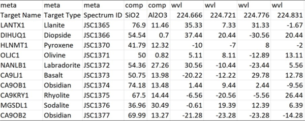
Python Hyperspectral Analysis Tool (PyHAT) Data Format ExampleScreenshot showing the simple data format used by the Python Hyperspectral Analysis Tool (PyHAT). Spectra are stored in rows of the table, along with their associated metadata and compositional information.
Python Hyperspectral Analysis Tool (PyHAT) Data Format Example
Python Hyperspectral Analysis Tool (PyHAT) Data Format ExampleScreenshot showing the simple data format used by the Python Hyperspectral Analysis Tool (PyHAT). Spectra are stored in rows of the table, along with their associated metadata and compositional information.
Python Hyperspectral Analysis Tool (PyHAT) Mineral Parameter Map Example - Jezero Crater, Mars
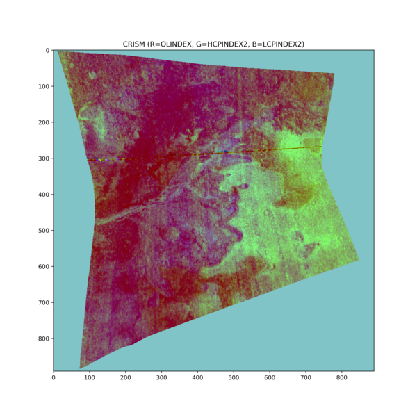
Python Hyperspectral Analysis Tool (PyHAT) Mineral Parameter Map Example - Jezero Crater, MarsThis figure shows an example mineral parameter map image generated using PyHAT. The area in this Compact Reconnaissance Imaging Spectrometer for Mars (CRISM) image is Jezero crater, the landing site of NASA's Mars Perseverance rover.
Python Hyperspectral Analysis Tool (PyHAT) Mineral Parameter Map Example - Jezero Crater, Mars
Python Hyperspectral Analysis Tool (PyHAT) Mineral Parameter Map Example - Jezero Crater, MarsThis figure shows an example mineral parameter map image generated using PyHAT. The area in this Compact Reconnaissance Imaging Spectrometer for Mars (CRISM) image is Jezero crater, the landing site of NASA's Mars Perseverance rover.
Python Hyperspectral Analysis Tool (PyHAT) Principal Component Analysis (PCA) Plot Example
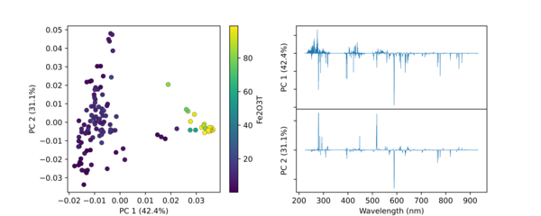
Python Hyperspectral Analysis Tool (PyHAT) Principal Component Analysis (PCA) Plot ExampleThis figure shows an example PCA plot generated using PyHAT. The input data were laser induced breakdown spectroscopy (LIBS) spectra. PyHAT was used to apply a baseline correction and normalization to the total intensity for each spectrum.
Python Hyperspectral Analysis Tool (PyHAT) Principal Component Analysis (PCA) Plot Example
Python Hyperspectral Analysis Tool (PyHAT) Principal Component Analysis (PCA) Plot ExampleThis figure shows an example PCA plot generated using PyHAT. The input data were laser induced breakdown spectroscopy (LIBS) spectra. PyHAT was used to apply a baseline correction and normalization to the total intensity for each spectrum.
Python Hyperspectral Analysis Tool (PyHAT) Principal Component Analysis K-Means Clustering Example
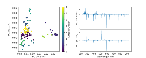
Python Hyperspectral Analysis Tool (PyHAT) Principal Component Analysis K-Means Clustering ExampleThis figure shows an example PCA plot generated using PyHAT. The input data were laser induced breakdown spectroscopy (LIBS) spectra. PyHAT was used to apply a baseline correction and normalization to the total intensity for each spectrum.
Python Hyperspectral Analysis Tool (PyHAT) Principal Component Analysis K-Means Clustering Example
Python Hyperspectral Analysis Tool (PyHAT) Principal Component Analysis K-Means Clustering ExampleThis figure shows an example PCA plot generated using PyHAT. The input data were laser induced breakdown spectroscopy (LIBS) spectra. PyHAT was used to apply a baseline correction and normalization to the total intensity for each spectrum.
Python Hyperspectral Analysis Tool (PyHAT) Outlier Identification Example
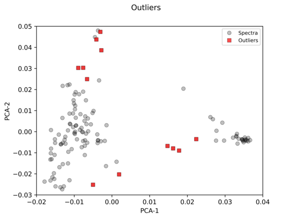
Python Hyperspectral Analysis Tool (PyHAT) Outlier Identification ExampleThis figure shows an example of outlier identification using PyHAT. The input data were laser induced breakdown spectroscopy (LIBS) spectra. PyHAT was used to apply a baseline correction and normalization to the total intensity for each spectrum. Dimensionality was then reduced using principal components analysis (PCA).
Python Hyperspectral Analysis Tool (PyHAT) Outlier Identification Example
Python Hyperspectral Analysis Tool (PyHAT) Outlier Identification ExampleThis figure shows an example of outlier identification using PyHAT. The input data were laser induced breakdown spectroscopy (LIBS) spectra. PyHAT was used to apply a baseline correction and normalization to the total intensity for each spectrum. Dimensionality was then reduced using principal components analysis (PCA).
Python Hyperspectral Analysis Tool (PyHAT) Partial Least Squares Cross Validation Example
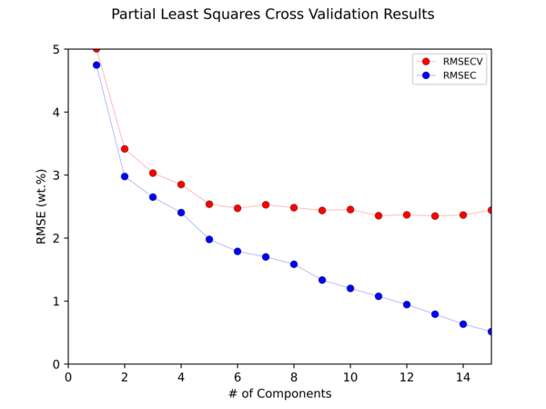
Python Hyperspectral Analysis Tool (PyHAT) Partial Least Squares Cross Validation ExampleThis figure shows the results of cross-validating a Partial Least Squares (PLS) model to predict the abundance of CaO in geologic targets using PyHAT. Cross validation is necessary to optimize the parameters of a regression algorithm to avoid overfitting.
Python Hyperspectral Analysis Tool (PyHAT) Partial Least Squares Cross Validation Example
Python Hyperspectral Analysis Tool (PyHAT) Partial Least Squares Cross Validation ExampleThis figure shows the results of cross-validating a Partial Least Squares (PLS) model to predict the abundance of CaO in geologic targets using PyHAT. Cross validation is necessary to optimize the parameters of a regression algorithm to avoid overfitting.
Python Hyperspectral Analysis Tool (PyHAT) Baseline Removal Plot Example
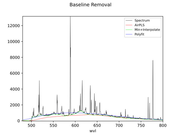
Python Hyperspectral Analysis Tool (PyHAT) Baseline Removal Plot ExampleThis figure shows an example spectrum plot generated using PyHAT. The black line is a laser induced breakdown spectroscopy (LIBS) spectrum of a basalt sample. The colored lines show the baseline estimated using several different algorithms.
Python Hyperspectral Analysis Tool (PyHAT) Baseline Removal Plot Example
Python Hyperspectral Analysis Tool (PyHAT) Baseline Removal Plot ExampleThis figure shows an example spectrum plot generated using PyHAT. The black line is a laser induced breakdown spectroscopy (LIBS) spectrum of a basalt sample. The colored lines show the baseline estimated using several different algorithms.
Python Hyperspectral Analysis Tool (PyHAT) Regression Example
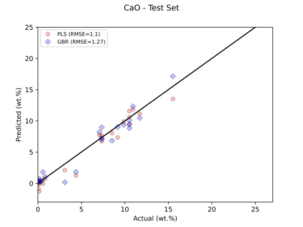
Python Hyperspectral Analysis Tool (PyHAT) Regression ExampleThis figure compares the results of two regression models to predict the abundance of CaO in geologic standards based on their laser induced breakdown spectroscopy (LIBS) spectra using PyHAT. The horizontal axis is the independently measured CaO abundance, the vertical axis is the abundance predicted by the models.
Python Hyperspectral Analysis Tool (PyHAT) Regression Example
Python Hyperspectral Analysis Tool (PyHAT) Regression ExampleThis figure compares the results of two regression models to predict the abundance of CaO in geologic standards based on their laser induced breakdown spectroscopy (LIBS) spectra using PyHAT. The horizontal axis is the independently measured CaO abundance, the vertical axis is the abundance predicted by the models.
Science and Products
Terrestrial Remote Sensing Data Ingestion with PyHAT (Python Hyperspectral Analysis Tool)
This work will make it easier to work with multiple terrestrial data sets in PyHAT, a USGS tool that enables machine learning analysis of spectral datasets
Python Hyperspectral Analysis Tool (PyHAT)
The Python Hyperspectral Analysis Tool (PyHAT) provides access to data processing, analysis, and machine learning capabilities for spectroscopic applications. It includes a GUI so you can get straight to analyzing data without writing any code. Or, if you are comfortable writing code, PyHAT can be imported just like any other Python package.
Python Hyperspectral Analysis Tool (PyHAT) Logo
This a version of the logo for the Python Hyperspectral Analysis Tool (PyHAT). It is intended for use in info boxes on the USGS website. The spectrum in the graphic is a laser induced breakdown spectroscopy spectrum, plotted on a logarithmic y axis to emphasize weaker emission peaks.
This a version of the logo for the Python Hyperspectral Analysis Tool (PyHAT). It is intended for use in info boxes on the USGS website. The spectrum in the graphic is a laser induced breakdown spectroscopy spectrum, plotted on a logarithmic y axis to emphasize weaker emission peaks.
Python Hyperspectral Analysis Tool (PyHAT) Data Format Example
Python Hyperspectral Analysis Tool (PyHAT) Data Format ExampleScreenshot showing the simple data format used by the Python Hyperspectral Analysis Tool (PyHAT). Spectra are stored in rows of the table, along with their associated metadata and compositional information.
Python Hyperspectral Analysis Tool (PyHAT) Mineral Parameter Map Example - Jezero Crater, Mars
Python Hyperspectral Analysis Tool (PyHAT) Mineral Parameter Map Example - Jezero Crater, MarsThis figure shows an example mineral parameter map image generated using PyHAT. The area in this Compact Reconnaissance Imaging Spectrometer for Mars (CRISM) image is Jezero crater, the landing site of NASA's Mars Perseverance rover.
Python Hyperspectral Analysis Tool (PyHAT) Principal Component Analysis (PCA) Plot Example
Python Hyperspectral Analysis Tool (PyHAT) Principal Component Analysis (PCA) Plot ExampleThis figure shows an example PCA plot generated using PyHAT. The input data were laser induced breakdown spectroscopy (LIBS) spectra. PyHAT was used to apply a baseline correction and normalization to the total intensity for each spectrum.
Python Hyperspectral Analysis Tool (PyHAT) Principal Component Analysis K-Means Clustering Example
Python Hyperspectral Analysis Tool (PyHAT) Principal Component Analysis K-Means Clustering ExampleThis figure shows an example PCA plot generated using PyHAT. The input data were laser induced breakdown spectroscopy (LIBS) spectra. PyHAT was used to apply a baseline correction and normalization to the total intensity for each spectrum.
Python Hyperspectral Analysis Tool (PyHAT) Outlier Identification Example
Python Hyperspectral Analysis Tool (PyHAT) Outlier Identification ExampleThis figure shows an example of outlier identification using PyHAT. The input data were laser induced breakdown spectroscopy (LIBS) spectra. PyHAT was used to apply a baseline correction and normalization to the total intensity for each spectrum. Dimensionality was then reduced using principal components analysis (PCA).
Python Hyperspectral Analysis Tool (PyHAT) Partial Least Squares Cross Validation Example
Python Hyperspectral Analysis Tool (PyHAT) Partial Least Squares Cross Validation ExampleThis figure shows the results of cross-validating a Partial Least Squares (PLS) model to predict the abundance of CaO in geologic targets using PyHAT. Cross validation is necessary to optimize the parameters of a regression algorithm to avoid overfitting.
Python Hyperspectral Analysis Tool (PyHAT) Baseline Removal Plot Example
Python Hyperspectral Analysis Tool (PyHAT) Baseline Removal Plot ExampleThis figure shows an example spectrum plot generated using PyHAT. The black line is a laser induced breakdown spectroscopy (LIBS) spectrum of a basalt sample. The colored lines show the baseline estimated using several different algorithms.
Python Hyperspectral Analysis Tool (PyHAT) Regression Example
Python Hyperspectral Analysis Tool (PyHAT) Regression ExampleThis figure compares the results of two regression models to predict the abundance of CaO in geologic standards based on their laser induced breakdown spectroscopy (LIBS) spectra using PyHAT. The horizontal axis is the independently measured CaO abundance, the vertical axis is the abundance predicted by the models.