
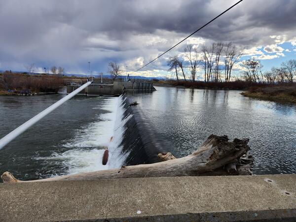
This is a photo of a dam in the lower Yakima River. Efforts to ameliorate the negative effects of diversion dams on aquatic species of concern are important in rivers where water withdrawal supports agricultural economies, and they are likely to become increasingly important with impending climate change.
Images
Explore images taken during Ecosystems' Land Change Science Program fieldwork and research.
Filter Total Items: 196
Dam in the lower Yakima River
This is a photo of a dam in the lower Yakima River. Efforts to ameliorate the negative effects of diversion dams on aquatic species of concern are important in rivers where water withdrawal supports agricultural economies, and they are likely to become increasingly important with impending climate change.
Survival Probabilities of Fish Through Canals Versus Dams
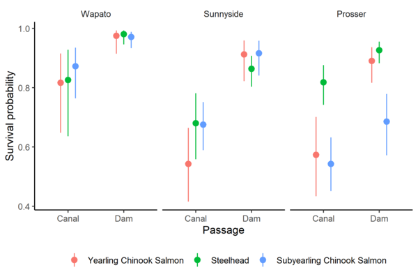
Survival Probabilities of Fish Through Canals Versus DamsSurvival probability estimates and 95% confidence intervals for yearling Chinook Salmon, juvenile steelhead, and subyearling Chinook Salmon at three diversion dams on the Yakima River, Washington.
Survival Probabilities of Fish Through Canals Versus Dams
Survival Probabilities of Fish Through Canals Versus DamsSurvival probability estimates and 95% confidence intervals for yearling Chinook Salmon, juvenile steelhead, and subyearling Chinook Salmon at three diversion dams on the Yakima River, Washington.
Nine Panel Plot of Fish Passage Entrainment vs Canal Flow
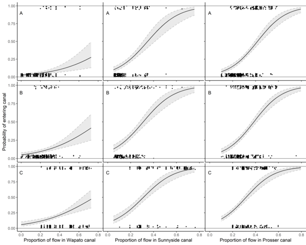
Nine Panel Plot of Fish Passage Entrainment vs Canal FlowEstimated relationship between entrainment probability and proportion of river flow entering canals at Wapato Dam, Sunnyside Dam, and Prosser Dam on the Yakima River, Washington. The relationships are shown at the mean total river flow for (A) yearling Chinook Salmon, (B) juvenile steelhead, and (C) subyearling Chinook Salmon.
Nine Panel Plot of Fish Passage Entrainment vs Canal Flow
Nine Panel Plot of Fish Passage Entrainment vs Canal FlowEstimated relationship between entrainment probability and proportion of river flow entering canals at Wapato Dam, Sunnyside Dam, and Prosser Dam on the Yakima River, Washington. The relationships are shown at the mean total river flow for (A) yearling Chinook Salmon, (B) juvenile steelhead, and (C) subyearling Chinook Salmon.

Discover Ecosystems
America’s diverse ecosystems are an asset to current and future generations by supporting economically and recreationally important fish, wildlife, and lands. Healthy ecosystems support people and nature, fostering prosperity and enjoyment for all.
America’s diverse ecosystems are an asset to current and future generations by supporting economically and recreationally important fish, wildlife, and lands. Healthy ecosystems support people and nature, fostering prosperity and enjoyment for all.

Discover Ecosystems
America’s diverse ecosystems are an asset to current and future generations by supporting economically and recreationally important fish, wildlife, and lands. Healthy ecosystems support people and nature, fostering prosperity and enjoyment for all.
By
Ecosystems Mission Area, Biological Threats and Invasive Species Research Program, Climate Adaptation Science Centers, Cooperative Research Units, Ecosystems Land Change Science Program, Environmental Health Program, Land Management Research Program, Species Management Research Program, Communications and Publishing

Fire In Ice Data Visualization Thumbnails
These three thumbnail illustrations represent three different data visualizations about USGS research on how wildfire affects the Juneau Icefield, Alaska. The upper left image of the Juneau Icefield represents a viz about where the icefield is located and where scientists collect data.
These three thumbnail illustrations represent three different data visualizations about USGS research on how wildfire affects the Juneau Icefield, Alaska. The upper left image of the Juneau Icefield represents a viz about where the icefield is located and where scientists collect data.

Beaufort Sea Data Visualization Thumbnails
These three thumbnail illustrations represent three different data visualizations about USGS research in the Beaufort Sea. The upper left image of an Arctic icebreaker and research vessel represents a viz about how sediment cores are collected.
These three thumbnail illustrations represent three different data visualizations about USGS research in the Beaufort Sea. The upper left image of an Arctic icebreaker and research vessel represents a viz about how sediment cores are collected.

USGS scientist holding clam
USGS scientist BJ Reynolds holds half of a Mercenaria spp. clamshell found by wading in shallow waters of South Tampa Bay, Florida.
USGS scientist BJ Reynolds holds half of a Mercenaria spp. clamshell found by wading in shallow waters of South Tampa Bay, Florida.

Cyanobacteria bloom in a shallow Michigan lake
Cyanobacteria bloom in a shallow Michigan lake during the fall of 2024. Photo by Leon Katona
Cyanobacteria bloom in a shallow Michigan lake during the fall of 2024. Photo by Leon Katona

Blue Carbon
Blue carbon refers to carbon captured in coastal and ocean ecosystems.
Blue carbon refers to carbon captured in coastal and ocean ecosystems.

Paul Henne and Computer Model
Paul Henne develops wildfire models using records of past climate and area burned. These models when combined with sedimentary records help scientists understand long-term interactions among climate, vegetation, people, and wildfire.
Paul Henne develops wildfire models using records of past climate and area burned. These models when combined with sedimentary records help scientists understand long-term interactions among climate, vegetation, people, and wildfire.

Sand Island, Palmyra Atoll
Sand Island, one of the first islands on the atoll to have successfully eradicated coconut palms, which were quickly replaced by a healthy Pisonia forest with abundant shorebird life.
Sand Island, one of the first islands on the atoll to have successfully eradicated coconut palms, which were quickly replaced by a healthy Pisonia forest with abundant shorebird life.

Western Lagoon Shoreline, Palmyra Atoll
A view of the shoreline with palm trees above bright blue water in the Western Lagoon, Palmyra Atoll.
A view of the shoreline with palm trees above bright blue water in the Western Lagoon, Palmyra Atoll.

Looking out to Sea, Palmyra Atoll
Calm, blue waters surround Palmyra Atoll. This view takes in the ocean scenery with a partial glimpse of lush green coastal vegetation on the landward side.
Calm, blue waters surround Palmyra Atoll. This view takes in the ocean scenery with a partial glimpse of lush green coastal vegetation on the landward side.

Palm-lined Coast, Palmyra Atoll
Crystal clear, turquoise waters surrounding a palm-lined beach on Palmyra Atoll.
Crystal clear, turquoise waters surrounding a palm-lined beach on Palmyra Atoll.

Driftwood on Palmyra Atoll
Driftwood lays partially submerged in clear blue water on sandy shore of Palmyra Atoll.
Driftwood lays partially submerged in clear blue water on sandy shore of Palmyra Atoll.

Dead Coconut Palms, Palmyra Atoll
A recently treated stand of coconut palms, standing and dead, which will naturally convert back to Pisonia forest, on Palmyra Atoll.
A recently treated stand of coconut palms, standing and dead, which will naturally convert back to Pisonia forest, on Palmyra Atoll.

Scenic Lagoon, Palmyra Atoll
Calm, clear and bright blue waters of a small shoreline lagoon on Palmyra Atoll.
Calm, clear and bright blue waters of a small shoreline lagoon on Palmyra Atoll.

Preparing sediment samples in the lab
Physical Scientist Michelle Leung and Research Geologist Natalie Kehrwald prepare sediment samples from Santa Fe Lake, New Mexico to analyze records of interactions between past fires and human activity over the last few thousand years.
Physical Scientist Michelle Leung and Research Geologist Natalie Kehrwald prepare sediment samples from Santa Fe Lake, New Mexico to analyze records of interactions between past fires and human activity over the last few thousand years.

Pisonia Forest, Palmyra Atoll
Pisonia forest where coconuts have already been eradicated on Palmyra Atoll. The forest is lush and green.
Pisonia forest where coconuts have already been eradicated on Palmyra Atoll. The forest is lush and green.

North Shore of Palmyra Atoll
A view of the sandy north shore of Palmyra Atoll, with a forested edge. Recently killed coconut palm trunks poke out of the forested area.
A view of the sandy north shore of Palmyra Atoll, with a forested edge. Recently killed coconut palm trunks poke out of the forested area.