
Introduction to Aquatic Remote Sensing
Welcome to our online introductory guide to Aquatic Remote Sensing! This guide is designed to serve as a jumping-off point to learn more about the field of Aquatic Remote Sensing. It includes a basic overview of what Aquatic Remote Sensing is, how remote sensing data are used, and basic aquatic optics.
This webpage includes five sections. Each of the first four sections include written material as well as pictures and figures, and ends with a video on the same topic. The fifth and final section is a collection of links and references to other useful aquatic remote sensing learning materials, data portals, etc.
Use the links below to jump to each section or go directly to view each video.
The material on this site was reviewed and improved by Dulcinea Avouris and Meredith McPherson. Peter Pearsall provided video and web editing. This guide was made possible by funding from the USGS Office of Employee Development (OED).
Introduction to Aquatic Remote Sensing
If you’ve ever looked at some water and noticed something about it, you have engaged in a rudimentary form of aquatic remote sensing. For example, if you’ve ever looked at your glass of water and seen some stuff floating in it and decided not to drink it, you have used observation to diagnose the color and clarity of your water and derived some information about that water.

Aquatic remote sensing is about translating optical properties of the water to information about what is in the water. Optical properties of the water, like clarity and color, are directly related to what is in the water. Water color and clarity are determined by the amount and types of particles and dissolved materials in the water. Three main things that dictate water color are 1) things and particles floating in the water (like sediments, plankton, seaweed, etc.), 2) dissolved molecules (especially dissolved organics, like tea), and 3) the water itself. Each of these materials absorbs some light and scatters or reflects the rest. In combination, these three categories of materials influence the apparent color of a water body that we observe. Understanding the relationship between the concentration of specific components and the apparent water color is the driving objective in the field of aquatic remote sensing science.
Remote Sensing refers to collecting information about a surface or structure remotely (i.e., without physically sampling it). When we talk about the field of remote sensing, usually people are referring to using satellites, aircraft, drones, and other platforms to collect data (often in the form of pictures and images) from afar.
There are two forms of remote sensing: active remote sensing, and passive remote sensing. Active sensors generate a source emission to send at the object of interest and then read the response signal to get information. Some examples include things like radar and LiDAR. Passive sensors measure the amount of energy (including visible light) from the sun naturally reflected or radiated off an object of interest, more like a traditional camera. Passive sensors also measure how much light in different wavelengths across the electromagnetic spectrum (i.e., different colors of light) is bouncing off an object. Altogether, passive sensors collect three dimensional images: an image with layers of spectral information in each pixel. We sometimes refer to this as an “image cube”. The x and y dimensions of this cube are the latitude and longitude of each pixel, and the z dimension is the spectral information. Passive remote sensing of water is the focus of this handbook and the accompanying video series.
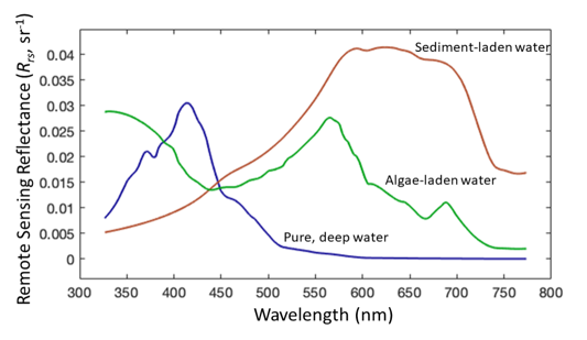
Passively collected spectral image data provides information on what’s on the surface of the earth–or in the case of aquatic remote sensing, what’s in the water–by quantifying the specific color signature of surface materials. We refer to these color signatures as “spectra,” because they quantify the light coming off a surface across the visible range of the electromagnetic spectrum. For example, clear, deep water appears blue to our eyes. If we look at a spectra of water, we see that it reflects some blue light and absorbs most light in other wavelengths. Similarly, muddy water appears brown to us. Spectra of sediment-laden water lets us quantify how brown some water is, which we can link to how much dirt is in the water using algorithms. This is the basis of aquatic remote sensing – in practice it gets slightly more complicated.
For a PDF of these slides, click here.
Aquatic Remote Sensing Data
In this section we will introduce the structure of remote sensing imagery, including dimensions and resolution of datasets. We’ll also introduce some of the most commonly used satellite sensors.
Aquatic remote sensing and optical data can be collected from a variety of different platforms. There’s satellite data, airborne data, drone data, and data collected from aboard ships. Passive imagery data is simply a picture of the earth’s surface that contains spectral information – that is, they measure the amount of light coming off a surface across the electromagnetic spectrum.
Types of Resolution
One of the most important things to understand about remote sensing data is the resolution of datasets. When deciding on a dataset to use and first approaching a problem, remote sensing scientists need to consider four different types of resolution. These are:
- Spatial resolution: the size of each pixel in the imagery.
- Temporal resolution: how often imagery is taken of the area of interest.
- Spectral Resolution: how many colors, or “bands” of light a sensor measures.
- Radiometric Resolution: how sensitive a sensor is to changes in brightness.
Spatial resolution is a concept you are probably already familiar with. Spatial resolution refers to the size of the pixels in an image. We describe it in terms of pixel size or Ground Sampling Distance (GSD). For example, we would say that Sentinel-2 has a GSD or pixel size of 10m.

Different sensors have a range of pixel sizes. For inland water bodies like lakes and rivers, higher spatial resolution is necessary to see the smaller-scale features. For open-ocean remote sensing, low spatial resolution is often helpful to see larger-scale patterns and deal with less data. Pixel size also affects the amount of signal available per pixel. Bigger pixels cover a larger area and therefore collect more light and signal from the target. Small pixels give a more detailed view and avoid averaging, but cover less area and therefore collect less light and signal.

Temporal resolution is also probably familiar to most scientists. Temporal resolution refers to how often something is observed. For remote sensing, we describe it in terms of frequency, revisit or repeat time. For example, we say that Landsat-8 has a 16-day revisit.
Temporal resolution of satellites ranges from every day to every few weeks for most passive sensors. Some satellites are constantly surveying and collecting data over one geographic area of Earth and have temporal resolution of less than a day. These are called “geostationary” satellites. Satellites that orbit the earth and collect data on a regular temporal cycle are more common and are “low earth orbit polar-orbiting” satellites. There are also “non-polar low earth” satellites, which collect data at specific areas of the surface only.

Spectral resolution is an important consideration for remote sensing. Spectral resolution refers to how many different types of light a sensor can measure, i.e., how many different colors a sensor can recognize. We talk about spectral resolution in terms of “bands” – a range of discrete wavelengths that a sensor measures light in. For example, a sensor with a “red band” might measure light in the red visible range, somewhere between 600-750 nm. Bands are defined by their center wavelength and their width.
The more bands a sensor measures, the higher the spectral resolution. Sensors may be “single-band” (i.e., they measure one band), “multi-band” or “multispectral” (i.e., they measure ~2-20 discrete bands), or “hyperspectral” (they measure hundreds of discrete bands). High spectral resolution sensors (hyperspectral) show the full spectrum of light in more detail. Lower spectral resolution sensors (single-band or multispectral) generally have higher signal to noise because they are taking in more light, but give a coarser view of the full spectrum.
Radiometric resolution is an important concept in remote sensing, but usually not as relevant a consideration as the first three types of resolution. Radiometric resolution refers to how much light can be detected by a sensor, i.e., how many different shades of a color a sensor can recognize. Where spectral resolution refers to how many colors a sensor can detect, radiometric resolution refers to how many shades of each of those colors a sensor can see. This is directly related to how much data can be collected and stored.
Radiometric resolution is therefore described in terms of bits (data storage). Lower resolution sensors see less shades and have less bits, higher resolution sensors see more shades and have more bits. For example, a low resolution 4-bit sensor has 16 available shades to measure and record. A high resolution 16-bit sensor has 65,536 available shades. Here is a USGS webpage with more information on radiometric resolution.

Each of these types of resolution is important to consider when deciding on a remote sensing dataset. For instance, if you’re interested in seeing how an algal bloom is evolving in a small estuary system, you might choose to use a satellite with a smaller pixel size and high frequency revisit. On the other hand, if you want to try and discriminate out different phytoplankton species in the coastal ocean, over a season, you might choose a sensor with lower spatial resolution but higher spectral resolution.
There are many other websites that introduce resolution types. Here are some:
| Mission Name | Aquatic Relevant Sensor | Spatial Resolution (highest) | Revisit | Spectral Resolution | Maintaining Agency | Start and end dates | Where to find data | More information |
| Landsat 4 and 5 | Multispectral Scanner (MSS) and Thematic Mapper (TM) | 57 x 79 m | 16 days | Multispectral | USGS/ NASA | 1982-2001 1985-2003 | https://earthexplorer.usgs.gov/ | |
| Landsat 8 | Operational Land Imager (OLI) | 30 m | 16 days | Multispectral | USGS/ NASA | 2013 | https://earthexplorer.usgs.gov/ | https://www.usgs.gov/landsat-missions/landsat-8 |
| Landsat 9 | Operational Land Imager (OLI-2) | 30 m | 16 days | Multispectral | USGS/ NASA | 2021 | https://earthexplorer.usgs.gov/ | https://www.usgs.gov/landsat-missions/landsat-9 |
MODIS (MODerate resolution Imaging Spectroradiometer) | MODIS (onboard satellites Terra and Aqua) | 1 km | 1 days | Multispectral | NASA | 1999- 2022 (Terra) 2002- 2022 (Aqua) | https://oceancolor.gsfc.nasa.gov/
|
|
| Sentinel 2 (A/B) | MultiSpectral Imager (MSI) | 10 m | 5 days | Multispectral | ESA | 2015 (S2A) 2016 (S2B) | https://dataspace.copernicus.eu/
| https://sentinel.esa.int/web/sentinel/missions/sentinel-2
|
| Sentinel 3 (A/B) | Ocean and Land Color Instrument (OLCI) | 300 m | 1-2 days | Multispectral | ESA | 2016 (S3A) 2028 (S3B) | https://dataspace.copernicus.eu/ | https://sentinels.copernicus.eu/web/sentinel/user-guides/sentinel-3-olci/overview |
PACE (Plankton, Aerosol, Cloud, ocean Ecosystem) | Ocean Color Instrument (OCI) | 1 km | 1-2 days | Hyperspectral | NASA | 2024 | https://pace.oceansciences.org/access_pace_data.htm | https://pace.oceansciences.org/home.htm |
For a more exhaustive list, Wikipedia has a list of earth observation satellites maintained by different agencies.
Note that this list doesn’t include commercial data. Some commercial groups like Planet and Maxar provide imagery for earth remote sensing applications and is free in some use cases.
It is important to note the units that data are in when downloading a product. This depends on both the processing level and the way the data are processed. Note that most US Level-2 data products (i.e., anything maintained by USGS or NASA) are reported as Remote Sensing Reflectance (Rrs), which has units of “per steradian” (sr-1). European products (i.e., anything maintained by the ESA) often come as Normalized Water-Leaving Reflectance (ρw) which is unitless. Rrs can be converted to ρw by multiplying by pi.
For a PDF of these slides, click here.
Basics of Aquatic Optics
In this section we will talk more about how water and different materials in water interact to change water color. For a far more detailed and complete overview of in-water optics, refer to the ocean optics handbook.
The main goal of remote sensing is to recognize materials on the surface of the earth and relay some information about them. For solid objects – like things on land or things floating on the surface of the water – this is relatively straightforward. But in aquatic environments the water body is a semi-transparent liquid mixture of different materials.
A large component of aquatic remote sensing is based on the concept that we can translate optical properties of water to information about what is in the water. The materials in water that contribute to the water color are known as optical constituents. Clarity and color are related to constituents in the water, and in aquatic remote sensing we aim to map and/or quantify the concentrations and types of those materials.
Each of these optical constituents interacts with light in two ways. Light is 1) absorbed, and 2) scattered. Absorption and scattering of light by materials in water are known as Inherent Optical Properties (IOP’s). These are the properties of the water that affect how it interacts with light. How much light is absorbed or scattered is different for different materials and varies across wavelengths. For example, water absorbs longer wavelengths (i.e., infrared and red) almost immediately, and shorter wavelengths (i.e., blue) last. This is why deep, pure water appears dark blue.

Introducing optical constituents to water changes the IOP’s of a water body. Major optical constituents within a water column that affect water color are:
- Particles
- Includes inorganic (i.e., suspended sediments) and organic (i.e., algae)
- The operational definition in oceanography is anything larger than 0.2 microns
- Organic dissolved materials
- The optically active (i.e., colored) portion of dissolved organic matter, known as Colored Dissolved Organic Matter (CDOM) – tea and coffee are both forms of CDOM that we drink!
- Oceanography definition is anything smaller than 0.2 microns.
- Water
- This also traditionally includes the inorganic component of dissolved materials (i.e., salts, anions, cations).
- Bubbles
- Primarily from wave action
For a more detailed description of optical constituents, see this page of the ocean optics webbook.
When only one constituent is having a direct effect on water color, retrievals (i.e., measurements via remote sensing) of that constituent are fairly straightforward. Retrievals of any one optical component become more complex as the number of optical constituents increases. Water bodies can be thought of as ranging in optical complexity. A water body with many different constituents contributing to the overall color and signal has high optical complexity; many rivers, lakes, estuaries, and the coastal ocean are considered optically complex. A water body with only one constituent (besides water) has low optical complexity. The open ocean–where algal chlorophyll is the only major optical constituent besides water–is a classic example.
Optically complex water bodies are where higher spectral resolution generally becomes more useful. This is because different constituents interact with different parts of the spectrum, so more spectral information can allow us to observe different things. This 2006 paper is a cool overview of how changes in water composition influence the apparent color of water bodies.
This leads us to the concept of Apparent Optical Properties (AOP’s). While IOP’s determine how light interacts with water, AOP’s refer to how that light is observed. The light bouncing out of and off of the water surface is what we perceive as water color. This is an AOP, and is quantified in different ways with different units, for example, Remote Sensing Reflectance (Rrs, per steradian (sr-1)) or Normalized Water-Leaving Reflectance (ρwN, unitless). AOP’s are determined by IOP’s (i.e., the color of water is determined by what’s in the water) but are also determined by changes in incoming light and direction of observation.
To avoid problems with variable lighting and glint, there are standardized methods for collecting water color measurements. There are also special considerations that need to be taken into account when the bottom is visible through the water column. If the benthos is your target, then it’s important to be able to remove the signal from the overlying water and constituents. If your target is the optical constituents in the water column, then the benthic reflectance needs to be removed from the signal.
For a PDF of these slides, click here.
Image Data Processing
This section presents an overview of the processing steps that scientists go through to turn remotely sensed satellite imagery into water quality maps.
This is a generalized overview. Different agencies (NASA, ESA, etc.) have different strategies for processing and disseminating data. Remote sensing data are stored and delivered in many file formats and structures. There is not a one-size-fits-all approach to any aspect of aquatic remote sensing data processing. We’ll talk generally about how data is processed, the major steps involved in processing, and where to find more information on algorithms and data products.

Remote sensing data at different processing steps is often referred to in terms of “levels.” Every time the data goes through an additional processing step, the product level increases. For example, Level 0 data is raw data directly from the sensor. Level 3 data products include things like chlorophyll, suspended sediment, or dissolved organics maps. We’ll work through each processing step and define the different levels of data.
Level-0 and Level-1: Data collection and Radiometric Calibration
Data is collected as Digital Number (Level 0). On the engineering side, there’s a lot that needs to be done to clean up data. Depending how data is collected, it may need to be stitched together, georectified (i.e., spatially referenced to a geographic coordinate system), or have other QA/QC steps applied, and finally it needs to be radiometrically calibrated. That is, the raw digital number needs to be converted to units of radiance (W/m2/sr) using a radiometric calibration established using known a standard. If you are collecting your own data from a drone or other accessible platform, you will need to do this processing yourself. If you are using satellite data, this step is done by the agency that operates the satellite.
Radiometric calibration is an important step for any sensor. Here’s an article by MicaSense (the makers of a drone-ready multispectral sensor) for more on what it is and why it’s so important. Once data is processed and in units of Radiance (W/m2/sr-1), we say it has been processed to Level-1. For satellite and other publicly distributed imagery, this is usually the first level of data that is available. Users may opt to download data at this level and apply their own downstream processing.
Level-2: Atmospheric correction
Once data is radiometrically calibrated and georectified, imagery must be atmospherically corrected. Various components of the atmosphere (i.e., gasses, particles, water vapor) interfere and dampen the signal from the earth’s surface. If you’re interested in aquatic targets, you need to atmospherically correct your data to remove the influence of the atmosphere on the signal. There are multiple software packages that are used for atmospheric correction, each replying on the same basic principles, but with different approaches in application.
A variety of atmospheric correction algorithms and packages have been developed for aquatic remote sensing. Here is a paper that compares some of the state-of-the-art atmospheric correction algorithms for Landsat-8 and Sentinel-2. A few of the most popular include ACOLITE, C2RCC (in the software SNAP). Sen2Cor (standalone)and L2gen in SeaDAS are also open-source, commonly used and relatively easy to work with. Other options include POLYMER (open-source) and some commercial corrections like FLAASH in ENVI. Level-2 data is also normalized to the incoming solar radiation, putting it in units of reflectance. Most US data products are reported as Remote Sensing Reflectance (Rrs), which has units of “per steradian” (sr-1). European products often come as Normalized Water-Leaving Reflectance (ρw) which is unitless. Rrs can be converted to ρw by multiplying by pi.
Most groups and agencies that publish remote sensing data provide a default atmospherically corrected Level-2 product using a specific atmospheric correction approach. These products are often optimized for land. While these corrections sometimes work for water, using an atmospheric correction for land may or may not perform with the same accuracy for aquatic targets. A common problem with using default, land-developed atmospheric corrections is that aquatic targets are under-corrected and there’s still atmospheric stuff contributing to the water leaving signal.
Another common problem in remote sensing is interference from clouds and glint. Clouds cannot be removed from imagery, and usually cloudy image data simply must be removed from further analysis. Some software packages are designed to work with cloudy data and can be used depending on your goals (i.e., DINEOF is designed to interpolate data gaps from clouds). Glint refers to when light reflects off water like a mirror, making it impossible to see the water color. This can be avoided by taking imagery at the right time of day to avoid problematic angles with the sun, but sometimes is inevitable. Like cloudy data, data affected by glint cannot usually be corrected in post-processing.
Level-3: derived products
Once imagery is atmospherically corrected, we can start to work with the data to generate some data products by applying retrieval algorithms to the Level 2 product. Retrieval algorithms are models that describe the relationship between the remote sensing spectral data and in-water constituents. Theoretically, any material that is optically active (i.e., contributes to the color of the water) can be retrieved.
There are some standard algorithms and data products that are publicly available (see the Resources section), but most water quality algorithms must be regionally and locally tuned to the water body of interest at the time of interest. This is because of how incredibly varied different water bodies are. For example, an algorithm for suspended sediments that is developed in a small lake with yellow clay will likely not perform with high accuracy in a large river with low levels of brown sediments.
There are many different algorithms for many different water quality variables, and there is no one accepted “correct” or “standard” way to retrieve water quality. But broadly there are three main approaches for recognizing spectral signals and relating them to what is in the water: spectral indices, data-driven, and semi-analytical. These three approaches are sometimes used individually, but quite often are combined with each other to create a retrieval algorithm or method.
Approaches for water quality retrievals
- Spectral Indices (band combinations)
- The overall premise of this approach is directly relating spectral features and information to information about what is in the water. For example: brighter, browner water corresponds to more suspended sediments, so higher reflectance in the 600-700nm range can be related to suspended sediment concentration. In optically simple environments like the open ocean, or in waters where one component is dominating the optical signal (i.e., is only one thing is influencing water color), indices are a powerful tool. However, indices are more difficult to rely on in optically complex waters where water color can be due to a variety of components. For example, a blue/green ratio index for chlorophyll might work well in optically simple environments where chlorophyll is the only optical constituent; however, in optically complex environments where sediments and dissolved organics also contribute to the signal, a blue/green index for chlorophyll will be less accurate.
- Data-driven
- Advances in technology have led to the collection of higher resolution imagery, and subsequently the creation of algorithms that leverage large datasets. Many algorithms leverage a data-driven approach to water quality retrievals, meaning they take advantage of a large dataset to look for spectral patterns associated with some material. Some examples include Machine Learning, Principle Least Squares Regression (PLSR), Principal Component Analysis (PCA). The accuracy and precision of those retrievals is often based on the scope of the training dataset. These are still empirical algorithms. These rely on sophisticated models to determine relationships between spectra and water quality variables but are still fundamentally reliant on in situ data.
- Semi-analytical
- Whereas spectral indices and data-driven approaches are purely empirically based, semi-analytical approaches use the physical relationships between light, water, and constituents. Semi-analytical algorithms use the rules of optics to solve for the inherent optical properties of a water body, and then translate those to the concentrations of optical constituents suspended in the water column. Such algorithms are analytically based and aim to solve a set of equations, but in practice also require empirical data, therefore making them “semi” analytical.
- The introduction in this paper gives a nice overview of semi-analytical algorithms.
Given the extensive processing that imagery must undergo before becoming a final data product, up to four types of data are required for building and validating retrieval algorithms: 1) remote sensing imagery viewing the surface, 2) surface-level radiometry is often needed to validate and fine-tune atmospheric correction, 3) in-water optical data is necessary if the inherent optics of the system need to be validated or understood, and 4) in-water samples are needed to create empirical relationships and validate final results. Fieldwork is often a required component of algorithm development, but there are also published global, local, and synthetic datasets that groups have compiled (e.g. GLORIA).
For a PDF of these slides, click here.
Resources
For viewing and downloading remote sensing data and data products:
- Earth Explorer: https://earthexplorer.usgs.gov/
- Earth Explorer contains NASA, USGS, and some ESA data available for download. You need an account but it’s free and fairly straightforward.
- Copernicus Data Space: https://dataspace.copernicus.eu/
- This is where ESA data products are officially available for access. They are also accessible through other platforms like Earth Explorer.
- NASA Ocean Color: https://oceancolor.gsfc.nasa.gov/
- This is where all NASA ocean color products are available for download, including products like ocean chlorophyll and sea surface temperature.
For viewing and creating remote sensing products online:
- NASA WorldView: https://worldview.earthdata.nasa.gov/
- This is NASA’s “one-stop-shop” for browsing remote sensing data products. It’s not actually exhaustive, and it’s not aquatic/marine specific, but it is fun and easy to use. Here's a YouTube video on Getting started with NASA Worldview.
- Copernicus Browser: https://browser.dataspace.copernicus.eu/
- A user-friendly interface and ESA's one-stop shop for creating spectral indices and doing some basic data manipulation, all without having to download anything. You can also search, filter, and download ESA imagery.
- Sentinel Playground: https://apps.sentinel-hub.com/sentinel-playground/
- Another ESA application, this is an easy way to view and explore data and download jpg/png images of different areas.
Free (no coding) software for working with remote sensing data:
- SNAP: https://step.esa.int/main/download/snap-download/
- SeaDAS: https://seadas.gsfc.nasa.gov/
- QGIS (more for spatial analysis): https://www.qgis.org/en/site/forusers/download.html
- Satellite-based analysis Tool for Rapid Evaluation of Aquatic environMents (STREAM) data portal: https://ladsweb.modaps.eosdis.nasa.gov/stream/map
- Water Information from SPace (WISP): https://apps.usgs.gov/wisp
Atmospheric Correction packages:
- Case 2 Regional Coast Color (C2RCC) in SNAP: https://c2rcc.org/
- ACOLITE: https://odnature.naturalsciences.be/remsem/software-and-data/acolite
- Sen2Cor in SNAP:https://step.esa.int/main/snap-supported-plugins/sen2cor/
- L2gen in SeaDAS: https://seadas.gsfc.nasa.gov/help-8.2.0/processors/ProcessL2gen.html
- POLYMER: https://www.hygeos.com/polymer
- FLAASH in ENVI: https://www.spectral.com/our-software/flaash/
Reference Materials for more learning:
- Ocean Optics Web Book: https://www.oceanopticsbook.info/
- The primary textbook for ocean optics, all online.
- Ocean Optics Course: https://misclab.umeoce.maine.edu/OceanOpticsClass2021/index.php/schedule/
- This course is taught every other summer by experts in the field of ocean optics and remote sensing at Bowdoin College. The 2021 course lectures were recorded and posted online at the link provided.
- NASA ARSET courses:
- International Ocean Colour Coordinating Group (IOCCG): https://ioccg.org/what-we-do/training-and-education/educational-links-and-resources/
- The IOCCG website, specifically the educational links and resources page, is a good place to find other training and is a great resource in itself.
- Papers referenced:
- Lehmann, M.K., Gurlin, D., Pahlevan, N. et al. GLORIA - A globally representative hyperspectral in situ dataset for optical sensing of water quality. Sci Data 10, 100 (2023). https://doi.org/10.1038/s41597-023-01973-y
- Goyens, C., Lavigne, H., Dille, A., Vervaeren, H. Using Hyperspectral Remote Sensing to Monitor Water Quality in Drinking Water Reservoirs. Remote Sens. 14(21), 5607 (2022). https://doi.org/10.3390/rs14215607
- Dierssen, H.M., Kudela, R.M., Ryan, J.P., Ziimmerman, R.C. Red and Black Tides: Quantitative Analysis of Water-Leaving Radiance and Perceived Color for Phytoplankton, Colored Dissolved Organic Matter, and Suspended Sediments. Limnol. Oceanogr., 51(6), 2646–2659 (2006). doi: 10.4319/lo.2006.51.6.2646