
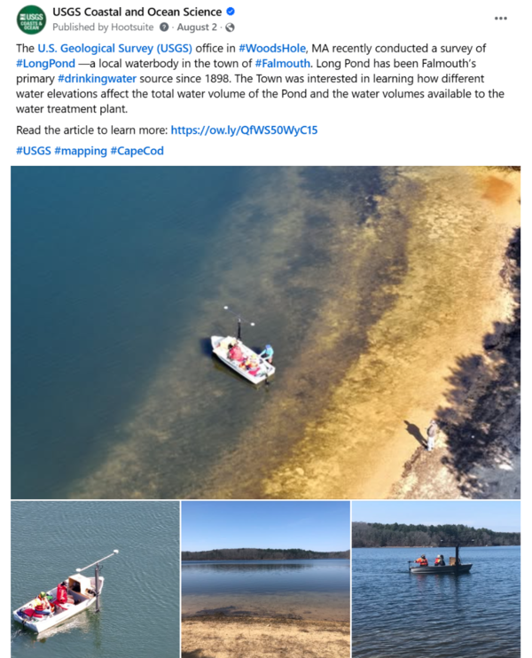
The USGS office in Woods Hole, MA recently conducted a survey of Long Pond—a local waterbody in the town of Falmouth. Long Pond has been Falmouth’s primary drinking water source since 1898.
Images
Coastal and Marine Hazards and Resources Program images.
Filter Total Items: 2415
Social Media: Long Pond mapping survey
The USGS office in Woods Hole, MA recently conducted a survey of Long Pond—a local waterbody in the town of Falmouth. Long Pond has been Falmouth’s primary drinking water source since 1898.
Summer 2025 Internship Presentations
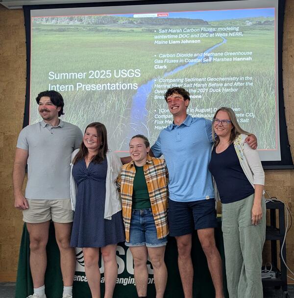
In August, the Woods Hole Coastal and Marine Science Center had four great presentations from summer interns discussing various aspects of salt marsh science!
In August, the Woods Hole Coastal and Marine Science Center had four great presentations from summer interns discussing various aspects of salt marsh science!
EPA/USGS Day of the 2025 Mashpee Wampanoag Tribe - Preserving Our Homelands Summer Camp
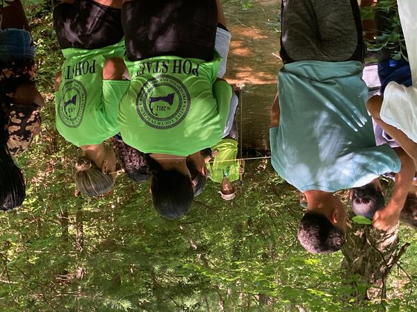
EPA/USGS Day of the 2025 Mashpee Wampanoag Tribe - Preserving Our Homelands Summer CampThe Environmental Protection Agency (EPA) and USGS prepared four activities for the Preserving Our Homelands Summer Camp on July 22nd. EPA hosted an air quality monitoring activity that involved the campers conducting tests and participating in a guided discussion about factors contributing to air quality and its implications on people and habitat.
EPA/USGS Day of the 2025 Mashpee Wampanoag Tribe - Preserving Our Homelands Summer Camp
EPA/USGS Day of the 2025 Mashpee Wampanoag Tribe - Preserving Our Homelands Summer CampThe Environmental Protection Agency (EPA) and USGS prepared four activities for the Preserving Our Homelands Summer Camp on July 22nd. EPA hosted an air quality monitoring activity that involved the campers conducting tests and participating in a guided discussion about factors contributing to air quality and its implications on people and habitat.
Example of a seasonally rotating beach of southern California
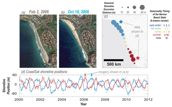
Example of a seasonally rotating beach of southern CaliforniaAn example seasonally rotating beach of southern California (Salt Creek Beach, 33.4788°N, 117.7237°W) showing (a,b) general patterns of rotation from satellite imagery, (c) spatial distribution of seasonal shoreline excursions (marker size) and timing of the shoreline seasonality (marker colour) from the STL and k-means results and (d) time series of shoreline posit
Example of a seasonally rotating beach of southern California
Example of a seasonally rotating beach of southern CaliforniaAn example seasonally rotating beach of southern California (Salt Creek Beach, 33.4788°N, 117.7237°W) showing (a,b) general patterns of rotation from satellite imagery, (c) spatial distribution of seasonal shoreline excursions (marker size) and timing of the shoreline seasonality (marker colour) from the STL and k-means results and (d) time series of shoreline posit
Estero de San Antonio on Bodega Bay
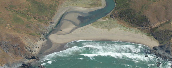
Aerial image of Estero de San Antonio on Bodega Bay, an example of a seasonally rotating pocket beach in California.
Aerial image of Estero de San Antonio on Bodega Bay, an example of a seasonally rotating pocket beach in California.
Social media for barrier island study
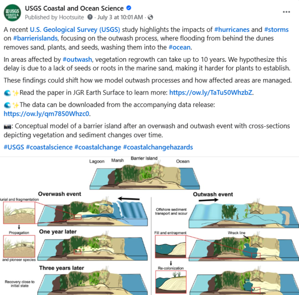
A recent USGS study highlights the impacts of #hurricanes and #storms on #barrierislands, focusing on the outwash process, where flooding from behind the dunes removes sand, plants, and seeds, washing them into the #ocean.
A recent USGS study highlights the impacts of #hurricanes and #storms on #barrierislands, focusing on the outwash process, where flooding from behind the dunes removes sand, plants, and seeds, washing them into the #ocean.
Social media for Superfund Site drone survey
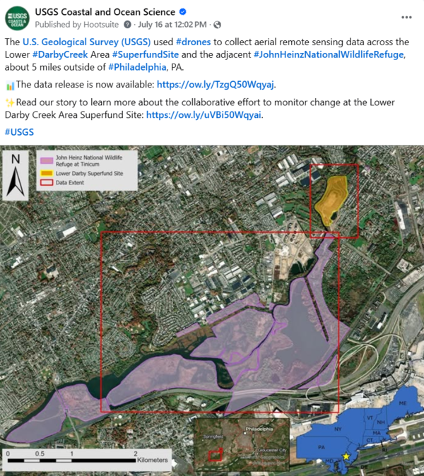
The USGS used #drones to collect aerial remote sensing data across the Lower #DarbyCreek Area Superfund Site and the adjacent #JohnHeinzNationalWildlifeRefuge, about 5 miles outside of #Philadelphia, PA. The data release is now available: https://doi.org/10.5066/P134HU3Y.
The USGS used #drones to collect aerial remote sensing data across the Lower #DarbyCreek Area Superfund Site and the adjacent #JohnHeinzNationalWildlifeRefuge, about 5 miles outside of #Philadelphia, PA. The data release is now available: https://doi.org/10.5066/P134HU3Y.
Social media for CRL model
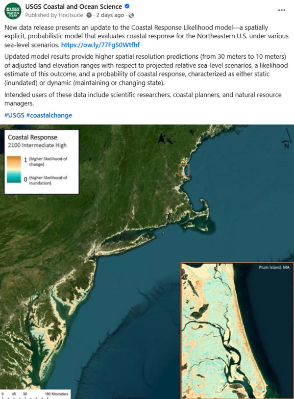
New data release presents an update to the Coastal Response Likelihood model—a spatially explicit, probabilistic model that evaluates coastal response for the Northeastern U.S. under various sea-level scenarios. https://doi.org/10.5066/P13JKJUT
New data release presents an update to the Coastal Response Likelihood model—a spatially explicit, probabilistic model that evaluates coastal response for the Northeastern U.S. under various sea-level scenarios. https://doi.org/10.5066/P13JKJUT

Mapping Nantucket Sound
Preparing equipment to map the geologic framework of Nantucket Sound, offshore Cape Cod, Massachusetts.
Preparing equipment to map the geologic framework of Nantucket Sound, offshore Cape Cod, Massachusetts.
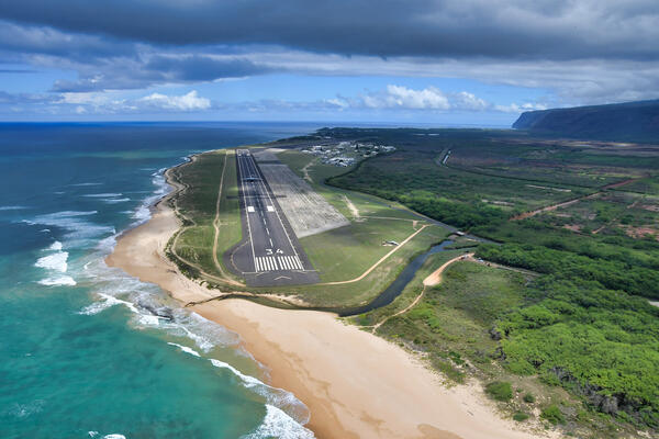
Pacific Missile Range Facility-Barking Sands in Hawai'i
Pacific Missile Range Facility-Barking Sands in Hawai'iPacific Missile Range Facility-Barking Sands in Hawai'i, operated by the U.S. Department of Defense.
Pacific Missile Range Facility-Barking Sands in Hawai'i
Pacific Missile Range Facility-Barking Sands in Hawai'iPacific Missile Range Facility-Barking Sands in Hawai'i, operated by the U.S. Department of Defense.

Banner image for Coastal Science Navigator
Banner image for the Coastal Science Navigator, an online gateway for users such as state and local planners, resources managers, consultants, and researchers to more easily gain access to USGS coastal science data, products, tools, and information.
Banner image for the Coastal Science Navigator, an online gateway for users such as state and local planners, resources managers, consultants, and researchers to more easily gain access to USGS coastal science data, products, tools, and information.
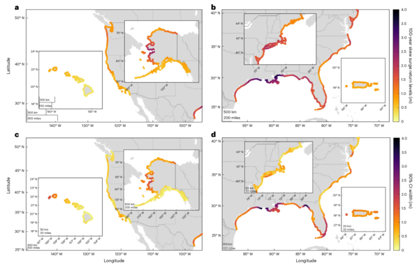
BAYEX predictions of 100-year storm surge return levels and associated 90% credible interval widths for the entire US coastline
BAYEX predictions of 100-year storm surge return levels and associated 90% credible interval widths for the entire US coastlineBAYEX predictions of 100-year storm surge return levels and associated 90% credible interval widths for the entire US coastline. From the study Observations reveal changing coastal storm extremes around the United States.
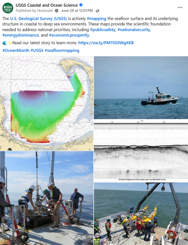
Social media for seafloor mapping article
The USGS is actively mapping the seafloor surface and its underlying structure in coastal to deep sea environments. These maps provide the scientific foundation needed to address national priorities, including #publicsafety, #nationalsecurity, #energydominance, and #economicprosperity.
The USGS is actively mapping the seafloor surface and its underlying structure in coastal to deep sea environments. These maps provide the scientific foundation needed to address national priorities, including #publicsafety, #nationalsecurity, #energydominance, and #economicprosperity.
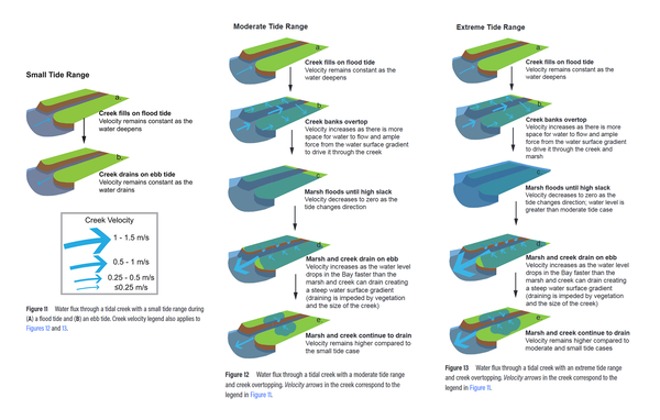
Charts depicting water flux through a tidal creek during flood and ebb tides
Charts depicting water flux through a tidal creek during flood and ebb tidesWater flux through a tidal creek with a small, moderate, and extreme tide range during (A) a flood tide and (B) an ebb tide. Creek velocity legend applies to all tide ranges.
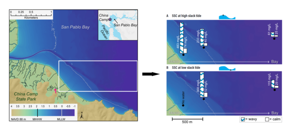
Maps showing China Camp Marsh study area with inset showing suspended sediment measurements
Maps showing China Camp Marsh study area with inset showing suspended sediment measurementsMap of study area: China Camp State Park and the adjacent shallows of San Pablo Bay. Black and gray bathymetry lines indicate the location of mean higher high water (MHHW) and mean lower low water (MLLW), respectively. Elevations in meters of those tidal datums are referenced to the North American Vertical Datum of 1988
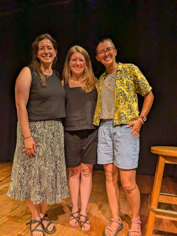
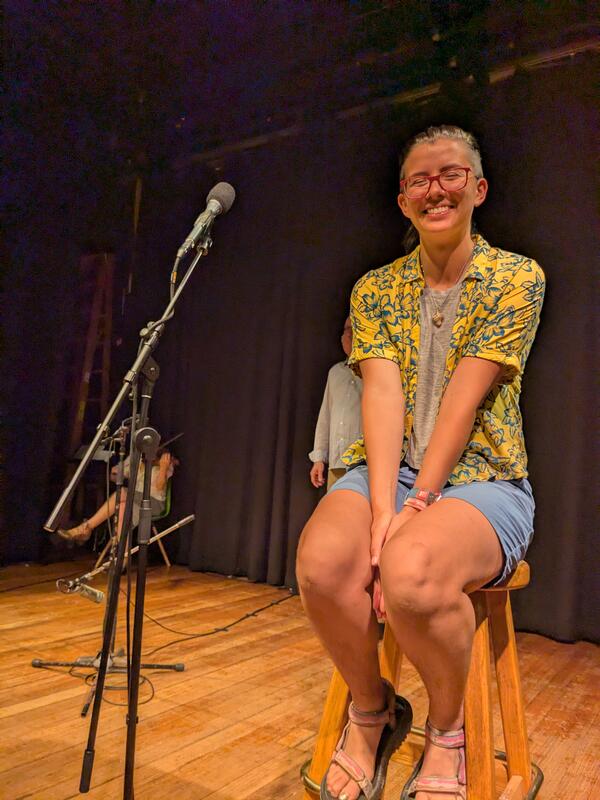
Science Storytelling
Non-profit organizations Transom Story Lab and Atlantic Public Media hosted a weekend-long science storytelling workshop called "Making Waves." It was attended by 11 scientists from scientific institutions throughout Woods Hole, Massachusetts, including USGS scientists Jin-Si Over, Ellen Lalk, and Sara Zeigler.
Non-profit organizations Transom Story Lab and Atlantic Public Media hosted a weekend-long science storytelling workshop called "Making Waves." It was attended by 11 scientists from scientific institutions throughout Woods Hole, Massachusetts, including USGS scientists Jin-Si Over, Ellen Lalk, and Sara Zeigler.
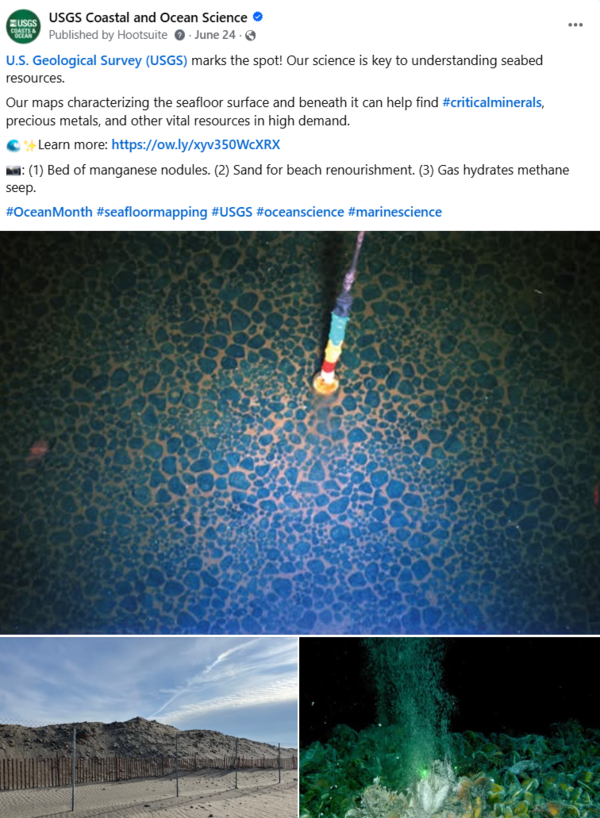
Social media for treasure maps article
USGS marks the spot! Our science is key to understanding seabed resources. Our maps characterizing the seafloor can help find #criticalminerals, precious metals, and other vital resources in high demand.
USGS marks the spot! Our science is key to understanding seabed resources. Our maps characterizing the seafloor can help find #criticalminerals, precious metals, and other vital resources in high demand.
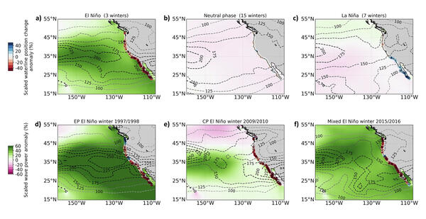
Hydrodynamic and morphological responses to El Nino Southern Oscillation phases along North America West Coast during winter 1997–2022
Hydrodynamic and morphological responses to El Nino Southern Oscillation phases along North America West Coast during winter 1997–2022Composites of hydrodynamic and morphological responses to (a–c) ENSO phases and (d–f) the strongest El Niño events during winter (DJF) over 1997–2022.

Study area overview with hydrodynamic forcings and beach morphology states
Study area overview with hydrodynamic forcings and beach morphology statesMap of the North American West Coast, the monitored coastline is shown in light yellow. Dashed boxes delineate the different subregions of the study area. Pie charts show the regional distribution of advancing/retreating waterline trends during 2000–2022 derived from the dataset presented in this study.
Science Storytelling
Non-profit organizations Transom Story Lab and Atlantic Public Media hosted a weekend-long science storytelling workshop called "Making Waves." It was attended by 11 scientists from scientific institutions throughout Woods Hole, Massachusetts, including USGS scientists Jin-Si Over, Ellen Lalk, and Sara Zeigler.
Non-profit organizations Transom Story Lab and Atlantic Public Media hosted a weekend-long science storytelling workshop called "Making Waves." It was attended by 11 scientists from scientific institutions throughout Woods Hole, Massachusetts, including USGS scientists Jin-Si Over, Ellen Lalk, and Sara Zeigler.

Examples of ecosystems that are chronically exposed to high levels of abiotic stress
Examples of ecosystems that are chronically exposed to high levels of abiotic stressPhotos of (a) coastal wetland, (b) coral reef, (c) dryland, and (d) alpine ecosystems. These ecosystems are chronically exposed to high levels of abiotic stress that approach physiological tolerance limits.