
Example of the Landsat Collection 2 Level-1 and Level-2 sample products from path 140 row 41, acquired on May 3, 2013. Left: Level-1 Top of Atmosphere. Middle: Level-2 Surface Reflectance. Right: Level-2 Surface Temperature.
Images
Explore the images on this page to learn more about the Landsat sensors, satellites and missions.
Filter Total Items: 399

Example of the Landsat Collection 2 products
Example of the Landsat Collection 2 Level-1 and Level-2 sample products from path 140 row 41, acquired on May 3, 2013. Left: Level-1 Top of Atmosphere. Middle: Level-2 Surface Reflectance. Right: Level-2 Surface Temperature.

Landsat 8 Surface Reflectance example
Left: Landsat 8 Top of Atmosphere reflectance image (bands 4,3,2) and Right: Landsat 8 atmospherically corrected surface reflectance image for an area in Nepal, path 141 row 40 acquired on May 3, 2013.
Left: Landsat 8 Top of Atmosphere reflectance image (bands 4,3,2) and Right: Landsat 8 atmospherically corrected surface reflectance image for an area in Nepal, path 141 row 40 acquired on May 3, 2013.

Example of Landsat 8 OLI/TIRS Collection 2 level-2 science products
Example of Landsat 8 OLI/TIRS Collection 2 level-2 science productsExample of the Landsat 8 OLI/TIRS Collection 2 level-2 science products. Left: Landsat 8 level-2 surface reflectance image. Right: Landsat 8 level-2 surface temperature image. The data was acquired on May 3, 2013 (path 140 row 41).

Landsat 7 Path 38 Row 31, Acquired March 29, 2013
On March 29-30, 2013, the Landsat Data Continuity Mission (later named Landsat 8) was in position under the Landsat 7 satellite. This provided opportunities for near-coincident data collection from both satellites.
On March 29-30, 2013, the Landsat Data Continuity Mission (later named Landsat 8) was in position under the Landsat 7 satellite. This provided opportunities for near-coincident data collection from both satellites.

Landsat 8 Path 38 Row 35, Acquired March 29, 2013
On March 29-30, 2013, the Landsat Data Continuity Mission (later named Landsat 8) was in position under the Landsat 7 satellite. This provided opportunities for near-coincident data collection from both satellites.
On March 29-30, 2013, the Landsat Data Continuity Mission (later named Landsat 8) was in position under the Landsat 7 satellite. This provided opportunities for near-coincident data collection from both satellites.

Landsat 7 Path 38 Row 35, Acquired March 29, 2013
On March 29-30, 2013, the Landsat Data Continuity Mission (later named Landsat 8) was in position under the Landsat 7 satellite. This provided opportunities for near-coincident data collection from both satellites.
On March 29-30, 2013, the Landsat Data Continuity Mission (later named Landsat 8) was in position under the Landsat 7 satellite. This provided opportunities for near-coincident data collection from both satellites.

Landsat 8 Path 38 Row 35
Landsat 8 image from Path 38 Row 35 near Peach Springs, Arizona. The image is shown as a false color composite using the shortwave infrared, near infrared, and red bands (Bands 6|5|4).
Landsat 8 image from Path 38 Row 35 near Peach Springs, Arizona. The image is shown as a false color composite using the shortwave infrared, near infrared, and red bands (Bands 6|5|4).

Boulder, Colorado - Landsat 8
Landsat 8’s first image captured the area where the Great Plains and Rocky Mountains meet in Colorado in March 2013. The natural-color image shows the coniferous forest of the mountains coming down to the dormant plains. Boulder, Colorado, sits in the middle of the image.
Landsat 8’s first image captured the area where the Great Plains and Rocky Mountains meet in Colorado in March 2013. The natural-color image shows the coniferous forest of the mountains coming down to the dormant plains. Boulder, Colorado, sits in the middle of the image.

Landsat 5 MSS Image of Michigan’s Upper Peninsula
This image of Michigan’s Upper Peninsula was captured by the Multispectral Scanner (MSS) instrument onboard the Landsat 5 satellite on January 7, 2013.
This image of Michigan’s Upper Peninsula was captured by the Multispectral Scanner (MSS) instrument onboard the Landsat 5 satellite on January 7, 2013.

Brown Marsh in Southeast Louisiana
Brown Marsh observed in southeastern Terrebonne Basin, La
Brown Marsh observed in southeastern Terrebonne Basin, La

Tile drain in intensive Corn Belt agriculture
A tile drain concentrates and transports irrigation water and the chemicals it contains to a stream.
A tile drain concentrates and transports irrigation water and the chemicals it contains to a stream.

Landsat 5 Captures MSS Data
The Multispectral Scanner (MSS) on board Landsat 5 satellite captured imagery of the southern Louisiana coastline on April 10, 2012, after the sensor was turned back on after being off for nearly a dozen years. This image is a portion of the scene from WRS-2 Path 23 Row 40. The MSS sensor collected nearly 15,000 scenes from 2012 to January 7, 2013.
The Multispectral Scanner (MSS) on board Landsat 5 satellite captured imagery of the southern Louisiana coastline on April 10, 2012, after the sensor was turned back on after being off for nearly a dozen years. This image is a portion of the scene from WRS-2 Path 23 Row 40. The MSS sensor collected nearly 15,000 scenes from 2012 to January 7, 2013.
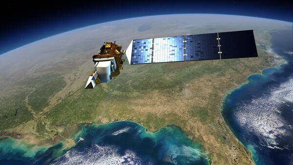
Image of Landsat 8 over the US
This illustration shows the Landsat 8 satellite in space over the southeastern United States.
This illustration shows the Landsat 8 satellite in space over the southeastern United States.

Tuscaloosa-Birmingham Tornado Scar, April 2011
The roughly west-east trail of destruction from the April 27, 2011, Tuscaloosa-Birmingham tornado is clearly visible in these Landsat images. This was one of 358 recorded tornadoes during the April 25-28, 2011, tornado outbreak, the most severe in U.S. history.
The roughly west-east trail of destruction from the April 27, 2011, Tuscaloosa-Birmingham tornado is clearly visible in these Landsat images. This was one of 358 recorded tornadoes during the April 25-28, 2011, tornado outbreak, the most severe in U.S. history.

Example of the Landsat Collection 2 Fractional Snow Covered Snow Science Product
Example of the Landsat Collection 2 Fractional Snow Covered Snow Science ProductExample of the Landsat Collection 2 Fractional Snow Covered Area (fSCA) Science Product showing an area in the Dixie National Forest in Utah on February 28, 2021 for tile h007V010. Left: Landsat Collection 2 U.S. Analysis Ready Data Surface Reflectance image, Middle: fSCA, and Right: Canopy Adjusted fSCA.

Landsat 5 image of Gascoyne, Australia
Landsat 5 image of Gascoyne, West Australia. The image was acquired on December 12, 2010.
Learn more about Landsat at www.usgs.gov/landsat
Landsat 5 image of Gascoyne, West Australia. The image was acquired on December 12, 2010.
Learn more about Landsat at www.usgs.gov/landsat

Example of Landsat Collection 2 Surface Temperature
Example of Landsat Collection 2 Surface TemperatureExample of Landsat Collection 2 Surface Temperature over the Tacoma, Washington area. Landsat 5 image aquired on October 6, 2010.
Example of Landsat Collection 2 Surface Temperature
Example of Landsat Collection 2 Surface TemperatureExample of Landsat Collection 2 Surface Temperature over the Tacoma, Washington area. Landsat 5 image aquired on October 6, 2010.

Landsat 5 image showing the Seattle, Washington area
Landsat 5 image showing the Seattle, Washington areaExample of the Landsat 4-5 TM Collection 2 level-1 product. This Landsat 5 image was acquired on October 6, 2010 near Seattle, Washington and is shown as a natural color composite using the red, green, and blue bands (bands 3,2,1).

Landsat Collection 2 Sample Data Example
Landsat 5 Thematic Mapper (TM) Collection 2 sample data example
Bands 5,4,3
Landsat 5 Thematic Mapper (TM) Collection 2 sample data example
Bands 5,4,3

Example of the Landsat Collection 2 Surface Reflectance product
Example of the Landsat Collection 2 Surface Reflectance productExample of the Landsat Collection 2 Level-2 Surface Reflectance science product over Seattle, Washington. Landsat 5 image acquired Oct 6, 2010 (bands 4,3,2)
Example of the Landsat Collection 2 Surface Reflectance product
Example of the Landsat Collection 2 Surface Reflectance productExample of the Landsat Collection 2 Level-2 Surface Reflectance science product over Seattle, Washington. Landsat 5 image acquired Oct 6, 2010 (bands 4,3,2)

Example of the Landsat 4-5 TM Collection 2 level-2 science products
Example of the Landsat 4-5 TM Collection 2 level-2 science productsExample of the Landsat 4-5 TM Collection 2 level-2 science products. Left: Landsat 5 level-2 surface reflectance image. Right: Landsat 5 level-2 surface temperature image. The data was acquired on October 6, 2010 (path 47 row 27).