
In 2017, the massive Mud Creek landslide buried a quarter-mile of the famous coastal route, California’s Highway 1, with rocks and dirt more than 65 feet deep. USGS monitors erosion along the landslide-prone cliffs of Big Sur, collecting aerial photos frequently throughout the year.
Images
Pacific Coastal and Marine Science Center images.
Filter Total Items: 1361

Mud Creek from June 13 to October 12, 2017
In 2017, the massive Mud Creek landslide buried a quarter-mile of the famous coastal route, California’s Highway 1, with rocks and dirt more than 65 feet deep. USGS monitors erosion along the landslide-prone cliffs of Big Sur, collecting aerial photos frequently throughout the year.
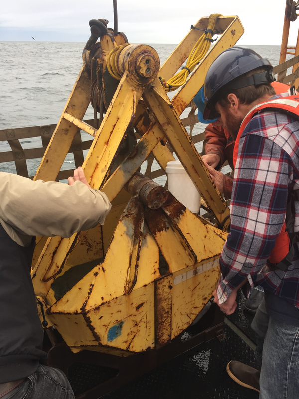
Examining bucket of seafloor sediment collected off southeast Alaska
Examining bucket of seafloor sediment collected off southeast AlaskaUSGS research geophysicist Danny Brothers (right) and colleagues examine the surface of a sediment grab sample just pulled onto the deck of the Canadian Coast Guard Ship John P. Tully. The sample was collected from the top of a mud volcano north of the border between southeast Alaska and British Columbia.

Collecting a piston core of seafloor sediment off British Columbia
Collecting a piston core of seafloor sediment off British ColumbiaScientists prepare to lower a piston corer off Haida Gwaii, British Columbia, to sample seafloor sediment near the Queen Charlotte-Fairweather fault. Expedition scientists are studying layers of sediment in the cores they collected to identify and determine ages of past earthquakes along the fault.

Sampling core fluid from sediment cores collected off southeast Alaska
Sampling core fluid from sediment cores collected off southeast AlaskaMary McGann (left, USGS) and Rachel Lauer (University of Calgary) sample pore fluids from sediment cores collected aboard the Canadian Coast Guard Ship John P. Tully along the Queen Charlotte-Fairweather fault offshore of southeast Alaska.

USGS geologist Carol Reiss examining hydrothermal vent sample
USGS geologist Carol Reiss examining hydrothermal vent sampleUSGS geologist Carol Reiss examining hydrothermal vent sample using hand lens. Sulfide-silicate minerals precipitate from 330°C mineral laden water venting along volcanically active spreading ridges.

USGS scientist Carol Reiss holding a hydrothermal vent sample
USGS scientist Carol Reiss holding a hydrothermal vent sampleUSGS scientist Carol Reiss holding a hydrothermal vent sample. The poster in the background is a scientific rendering by Véronique Robigou (then at University of Washington) of a hydrothermal vent deposit with the submersible Alvin drawn to scale.

Skagit Bay bathymetry
Skagit Bay bathymetry

McKelvey Building on the Menlo Park USGS campus
Construction of the McKelvey Building, or Building 15, was completed in the mid-1990s on the USGS Western Region campus in Menlo Park, California. It houses many different USGS teams, such as Pacific Coastal and Marine Science Center, Water Science Center, and Volcano Science Center, and features many state-of-the-art laboratories.
Construction of the McKelvey Building, or Building 15, was completed in the mid-1990s on the USGS Western Region campus in Menlo Park, California. It houses many different USGS teams, such as Pacific Coastal and Marine Science Center, Water Science Center, and Volcano Science Center, and features many state-of-the-art laboratories.

X-ray diffractometer
USGS research oceanographer Amy Gartman waits for an X-ray diffractometer to analyze samples of hydrothermal sulfide minerals.
USGS research oceanographer Amy Gartman waits for an X-ray diffractometer to analyze samples of hydrothermal sulfide minerals.

Scott Creek area of California coast
Aerial photograph looking north, Scott Creek Beach in distance, along the California coast near Davenport.
Aerial photograph looking north, Scott Creek Beach in distance, along the California coast near Davenport.

Seafloor crust, Marshall Islands
Cross section of a seafloor crust (AKA, ferromanganese or cobalt-rich crusts) from the Marshall Islands collected at almost 2,000 meters depth.
Cross section of a seafloor crust (AKA, ferromanganese or cobalt-rich crusts) from the Marshall Islands collected at almost 2,000 meters depth.

San Gregorio Beach and Creek
Flow from San Gregorio Creek in San Gregorio, California is often blocked by a natural sand levee when the flow is not strong enough to push through to the Pacific Ocean.
Flow from San Gregorio Creek in San Gregorio, California is often blocked by a natural sand levee when the flow is not strong enough to push through to the Pacific Ocean.

Reef-mounted instruments
Instrument package mounted to the seaward slope of a coral reef off southwestern Puerto Rico.
Instrument package mounted to the seaward slope of a coral reef off southwestern Puerto Rico.

Mapping squadron
Left to right: In July 2017 Tim Elfers (USGS), Hannah Drummond (WA State Dept. of Ecology), Heather Weiner (WA State Dept. of Ecology), Andrew Stevens (USGS), and Andy Ritchie (USGS) used handheld computers and backpack-mounted GPS equipment to record topography along a beach near the mouth of the Elwha River.
Left to right: In July 2017 Tim Elfers (USGS), Hannah Drummond (WA State Dept. of Ecology), Heather Weiner (WA State Dept. of Ecology), Andrew Stevens (USGS), and Andy Ritchie (USGS) used handheld computers and backpack-mounted GPS equipment to record topography along a beach near the mouth of the Elwha River.

Location of Mud Creek slide
Lead-in to the Mud Creek slide UAS (drone) footage, Big Sur, California, July 19. 2017.
Lead-in to the Mud Creek slide UAS (drone) footage, Big Sur, California, July 19. 2017.

Small computer that controls video cameras above beach in Santa Cruz
Small computer that controls video cameras above beach in Santa CruzThe small computer, or “micro-controller,” at the bottom of this photo controls the operation of two video cameras mounted on the 10-story Dream Inn hotel in Santa Cruz, California.

Big Sur Coast
Near San Simeon, view looks north up Highway 1 along the California coast toward Big Sur.
Near San Simeon, view looks north up Highway 1 along the California coast toward Big Sur.

Drone’s-eye views of the toe of the Mud Creek landslide
Drone’s-eye views of the toe of the Mud Creek landslideDrone’s-eye views of the toe of the Mud Creek landslide, from videos shot by Shawn Harrison on July 12, 2017
Drone’s-eye views of the toe of the Mud Creek landslide
Drone’s-eye views of the toe of the Mud Creek landslideDrone’s-eye views of the toe of the Mud Creek landslide, from videos shot by Shawn Harrison on July 12, 2017

Preliminary seafloor bathymetry collected by the USGS on July 11, 2017
Preliminary seafloor bathymetry collected by the USGS on July 11, 2017Preliminary seafloor bathymetry (shown in colors) collected by the USGS research vessel Parke Snavely on July 11, 2017. Relative depths shown in color, superimposed on a shaded-relief map from the June 26 USGS air-photo survey. Note white data gap next to the shore where water was too shallow for the Snavely to map.

Big Sur Landslide, July 7, 2017
USGS scientists continue to monitor the slide by collecting imagery every couple of weeks, weather permitting. Pilot Bob Van Wagenen, contracted through the Department of the Interior’s Office of Aviation Services, takes air photos for Jon Warrick’s Big Sur Landslide team, flying out of the Watsonville Municipal Airport in a Cessna 182R.
USGS scientists continue to monitor the slide by collecting imagery every couple of weeks, weather permitting. Pilot Bob Van Wagenen, contracted through the Department of the Interior’s Office of Aviation Services, takes air photos for Jon Warrick’s Big Sur Landslide team, flying out of the Watsonville Municipal Airport in a Cessna 182R.

Streamer depth control device, or bird
The Geospace Navigator bird is a streamer depth control device, used with a high-resolution seismic system to regulate and record the depth of the streamer.
The Geospace Navigator bird is a streamer depth control device, used with a high-resolution seismic system to regulate and record the depth of the streamer.