Images

Time to get our hands dirty! Paleoclimate researchers study sediment cores, which are accumulated layers of mud and dead plant material collected in a long tube, to learn about what the climate and environment of the past was like.

Two species of eyed ostracodes that exhibit eye tubercles and inhabit continental shelf environments. Eye tubercles are externally visible semi-globular structures of the calcareous shell, one in each of the two valves.

A bird biologist holds a ruby-throated hummingbird in the hand. 

Climate change data from the USGS National Climate Change Viewer tool is shown by US state and county for the contiguous US.

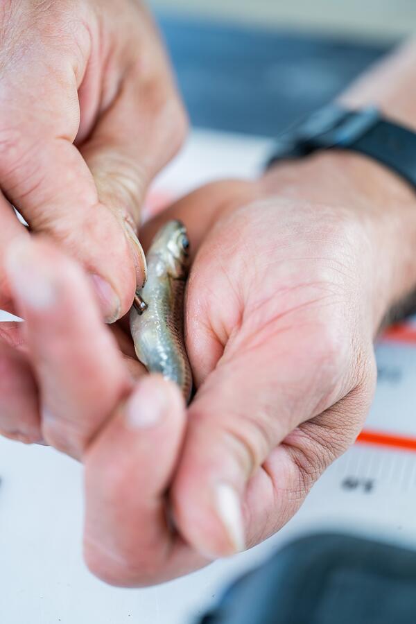
Ted Castro-Santos of the S.O. Conte Research Laboratory implants a small pit tag into a juvenile American shad before release it into the canal at Turners Falls, MA. 

A scientist looks at a Ponderosa Pine tree core using a rotary measuring stage. Credit: Becky Brice, USGS.

One Green River Ponderosa Pine sample after mounting and sanding lab procedures. Credit: Becky Brice, USGS.

Slide 2: Once a region of interest is selected, the control options are displayed on the left-hand side of the application. These control which climate variable, month, model, scenario, and time period are displayed in the map and charts.

Slide 3: The dropdown menus on the left-hand side contain all the variable options that can be individually selected in the NCCV.

Slide 4: On the right-hand side menu, the Model Agreement screen option displays the range of change simulated by the group of climate models with additional information on if the projected change is consistent in sign among the models and if the projections are statistically significant.

Slide 7: From the right-hand side menu, the Scatter Plot allows you to visualize the spread of all the models for two variables. This can be useful in understanding the relationship between variables in the projections, such as warm-and-wet or warm-and-dry for temperature and precipitation.

Slide 8: The National Climate Change Viewer (NCCV) application includes downloadable PDF reports, CSV data files, or JavaScript JSON data files for every state, county, and watershed.

Slide 1: Upon opening the National Climate Change Viewer (NCCV) you must select a region of interest to display the charts by either navigating and clicking on the map or selecting a location from the dropdown menu option on the left-hand side.

Slide 5: From the right-hand side menu, the Ensemble Timeseries Chart summarizes the group of models with a median line and range band, displaying the projected change through time.

Slide 6: From the right-hand side menu, the Data Table view displays the projected change for all models in tabular form. Clicking on the top row of the table allows you to sort the columns in ascending or descending order.

A USGS scientist maintaining a soil monitoring station in the Elk Mountains of Colorado. Soils play an important role in the global carbon cycle. USGS scientists measure and map soil carbon storage in many public lands of the southwestern U.S.

A scenic view of Gothic Mountain in the Elk Mountains of Colorado. USGS scientists captured this photo while collecting soil sample data in the area.

A view of Gothic Mountain from the Rocky Mountain Biological Laboratory research meadow in Gothic, Colorado.

A forest trail meanders through a grove of Aspen trees in Colorado during early autumn.

A USGS scientist preparing a soil monitoring station for winter, with a view of Mt. Baldy in the Colorado Elk Mountains.

A stunning farewell to the field expedition in Dinosaur National Monument with early morning sunshine gleaming off the riverside cliffs. Credit: Becky Brice, USGS.