Images

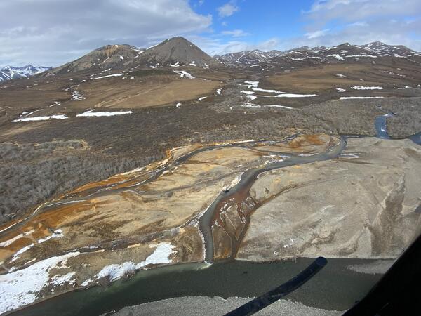
The USGS Water Resources Mission Area will assess water availability based on these core components of water supply and demand. 

Physical Scientist Molly Huber of the Florence Bascom Geoscience Center examines tree roots in a location where a root cookie was recently cut.

Molly was there as part of a stream habitat/riparian assessment at Orson Creek in south central Pennsylvania.

#RecreateWithUSGS is a national photo contest to raise awareness of the importance of USGS water data collected on public lands where people recreate in, on, and around water. Participate in this national photo contest and share your photo with us. Post on Instagram using #RecreateWithUSGS and tag @USGS_Water. The contest is open from June 12th - August 20th, 2023.

Orange streams are increasingly common in the Brooks Range of northern Alaska. The orange stream color reflects oxidized iron, but also often indicates elevated heavy metal concentrations. Our ongoing study aims to document these occurrences and the timing of their onset.

Orange streams are increasingly common in the Brooks Range of northern Alaska. The orange stream color reflects oxidized iron, but also often indicates elevated heavy metal concentrations. Our ongoing study aims to document these occurrences and the timing of their onset.

Orange streams are increasingly common in the Brooks Range of northern Alaska. The orange stream color reflects oxidized iron, but also often indicates elevated heavy metal concentrations. Our ongoing study aims to document these occurrences and the timing of their onset.

Photo of Blake Dudding, USGS, performing a survey on the banks of Lake Anna, Virginia 

USGS hydrographer Kristopher Ross makes an acoustic streamflow measurement from a cableway at streamgage 10308200 East Fork Carson River below Markleeville Creek, near Markleeville, CA. This station was recently nominated to be a part of the new Federal Priority Streamgage network design.​

Regional water availability assessment basins, as of 2023. USGS is conducting regional water availability assessments in medium-sized watersheds throughout the US.  These assessments are designed to capture a range of conditions in major drivers of water availability.

The USGS Water Resources Mission Area will assess water availability based on these core components of water supply and demand. 

USGS Scientist Brendan Foster taking and sealing an algal sample on a dock at Lake Anna, Virginia.

Image of pipettors used in the laboratory. Pipettes are stored on charging docking stations. 

Conceptual illustration showing how USGS's Next Generation Water Observing System will enhance the spatial and temporal monitoring of water within reference basins and larger hydrologic regions in all U.S. states and territories.

Eared grebes in a courtship behavior in the Great Salt Lake. They are one of many migratory birds in the Great Basin that rely on terminal lakes and wetlands in the area to stop rest and feed. 

A split-panel map of Salt Lake City, Utah, highlighting the Great Salt Lake, shows 2006 Landsat imagery on the left side panel and 2006 NLCD, with colorized legend of land use classes, on the right. The animation displays a slider being used to switch between the two different datasets, revealing the land cover classes shown in Landsat imagery.

Thumbnail image for a short video on the importance of USGS gages. This image shows three unique photos of USGS gages.

Image shows equipment for analysis of targeted and non-targeted organic contaminants at the OGRL located at the KS WSC. 

Stacked bar chart of 1990-2019 agriculture, domestic, and industry freshwater withdrawals in the U.S., estimated by the World Bank. In all years, industry withdraws the most freshwater, followed by agriculture and domestic. From 2006 to 2010, industrial water dropped 5,000 cubic kilometers, then remained low.

Animation of five satellite images of the Tanana River in Alaska. The imagery is colored in shades of blue to show the degree of confidence that water is present. Two scatter plots show positive pairwise relationships between satellite river elevation and satellite river width and satellite streamflow.

A tile map of the U.S. with lollipop charts for each state that show differences in forest area magnitude, in squared kilometers, from the 35-year mean (1985-2020) across the contiguous United States (CONUS). Positive differences are shown in forest green lollipops and negative differences are shown in burnt orange lollipops.

Six lollipop charts highlight deviations in maximum percent ice cover on the five Great Lakes (Lake Michigan, Lake Erie, Lake Superior, Lake Huron, and Lake Ontario) from 1973-2023. The difference in lake ice cover is shown for each lake and across the entire system compared to the 50-year mean (1973-2023).